Chapter 10 Whole Genome or Exome Sequencing

This chapter is in a beta stage. If you wish to contribute, please go to this form or our GitHub page.

10.1 Learning Objectives

The learning objectives for this course are to explain the use and application of Whole Genome Sequencing (WGS) and Whole Exome Sequencing (WES/WXS) for genomics studies, outline the technical steps in generating WGS/WXS data, and detail the processing steps for analyzing and interpreting WGS/WXS data.

To familiarize yourself with sequencing methods as a whole, we recommend you read our chapter on sequencing first.

10.2 WGS and WGS Overview

The difference between WGS and WXS sequencing is whether or not the open reading frames and thus coding regions are targeted in sequencing. WGS attempts to sequence the whole genome, while for WXS only exons with open reading frames are targeted for sequencing. Both of these methods can be massively beneficial for studying rare and complex diseases.

Thus, whole genome sequencing is a technique to thoroughly analyze the entire DNA sequence of an organism’s genome. This includes sequencing all genes both coding and non-coding and all mitochondrial DNA. WGS is beneficial for identifying new and previously established variants related to disease and the regulatory elements of the genome including promoters, enhancers, and silencers. Increasingly non-coding RNAs have also been identified to play a functional role in biological mechanisms and diseases. In order to learn more about the non-coding regions of the genome, WGS is necessary.

Alternatively whole exome sequencing is used to sequence the coding regions of an organism’s genome. Although non-coding regions can sometimes reveal valuable insights, coding regions can be a useful area of the genome to focus sequencing methods on, since changes in a protein coding sequence of the genome generally have more information known about them. Often protein coding sequences can have more clearly functional changes - like if a stop codon is introduced or a codon is changed to a predictable amino acid. This can more easily lead to downstream investigations on the functional implications of the protein affected.

10.3 Advantages and Disadvantages of WGS vs WXS

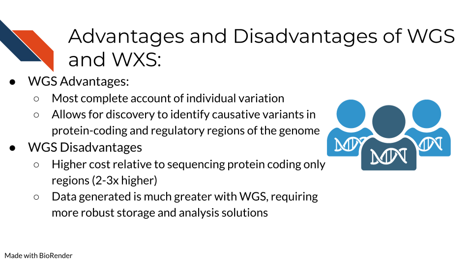
We more thoroughly discuss how to choose DNA sequencing methods here in the previous chapter, but we will briefly cover this here. Alternatives to WGS include Whole Exome Sequencing (WES/WXS), which sequences the open reading frame areas of the genome or Targeted Gene Sequencing where probes have been designed to sequence only regions of interest. The main advantages of WGS include the ability to comprehensively analyze all regions of a genome, the ability to study structural rearrangements, gene copy number alterations, insertions and deletions, single nucleotide polymorphisms (SNPs), and sequencing repeats. Some disadvantages include higher sequencing costs and the necessity for more robust storage and analysis solutions to manage the much larger data output generated from WGS.

10.4 WGS/WXS Considerations

Some important considerations for WGS/WXS include:

• What genome you are studying and the size of this genome. Included in this considerations is whether this genome has been sequenced before and you will have a “reference” genome to compare your data against or whether you will have to make a reference genome yourself. This bioinformatics resource provides a great overview of genome alignment.
• The depth of coverage for sequencing is an important consideration. The typical recommendation for WGS coverage is 30x, but this is on the lower side and many researchers find it does not provide sufficient coverage compared to 50x. Illumina has an infographic that explains this information
• The tissue source and whether genetic alterations were introduced during processing are important. Fixation for formalin-fixed paraffin embedded (FFPE) can introduce mutations/genetic changes that will need to be accounted for during data analysis. This page from Beckman addresses many of the questions researchers often have about utilizing FFPE samples for their sequencing studies.
• The library preparation method of DNA amplification via PCR is very important as PCR can often introduce duplicates that interfere with interpreting whether a mutant gene is truly frequent or just over amplified during sequencing preparation. Illumina provides a comparison of using PCR and PCR-free library preparation methods on their website.

10.4.1 Target enrichment techniques

For WXS or other targeted sequencing specifically (so not relevant to WGS data), what methods were used to enrich for the targeted sequences? (Which is the entire exome in the case of general WXS) These methods are generally summarized into two major categories: Hybridization based and amplicon based enrichment.

- [Hybridization based enrichment](https://www.paragongenomics.com/target-enrichment/). This includes a variety of widely used methods that we will broadly categorize in two groups: Array-based and In-solution:
  - [Array-based capture](https://en.wikipedia.org/wiki/Exome_sequencing#:~:text=Target%2Denrichment%20strategies-,Array%2Dbased%20capture,-In%2Dsolution%20capture) uses microarrays that have probes designed to bind to known coding sequences. Fragments that do not bind to these probes are washed away, leaving the sample with known coding sequences bound and ready for PCR amplification [@Hodges2007; @Turner2009].
  - [In-solution capture](https://en.wikipedia.org/wiki/Exome_sequencing#In-solution_capture) has become more popular in recent years because it [requires less sample DNA than array-base capture](https://sequencing.roche.com/global/en/article-listing/what-is-ngs-target-enrichment-and-why-is-it-important.html). To enrich for coding sequences, in-solution capture has a pool of custom probes that are designed to bind to the coding regions in the sample. Attached to these probes are beads which can be physically separated from DNA that is not bound to the probes (this should be the non-coding sequences) [@Mamanova2010].  
- [PCR/Amplicon based enrichment](https://www.ncbi.nlm.nih.gov/pmc/articles/PMC9318977/) requires even less sample than the other two strategies and so is ideal for when the amount of sample is limited or the DNA has been otherwise processed harshly (e.g. with paraffin embedding). Because the other two enrichment methods are done after PCR amplification has been done to the whole genomic DNA sample, its thought that this method of selective PCR amplification for enrichment can result in more uniformly amplified DNA in the resulting sample. However this is less suitable the more gene targets you have (like if you truly need to sequence all of the exome) since amplicons need to be designed for each target. Overall it is much more affordable of a method. There are several variations of this method that are [discussed thoroughly by @Singh2022](https://www.ncbi.nlm.nih.gov/pmc/articles/PMC9318977/).

10.5 DNA Sequencing Pipeline Overview

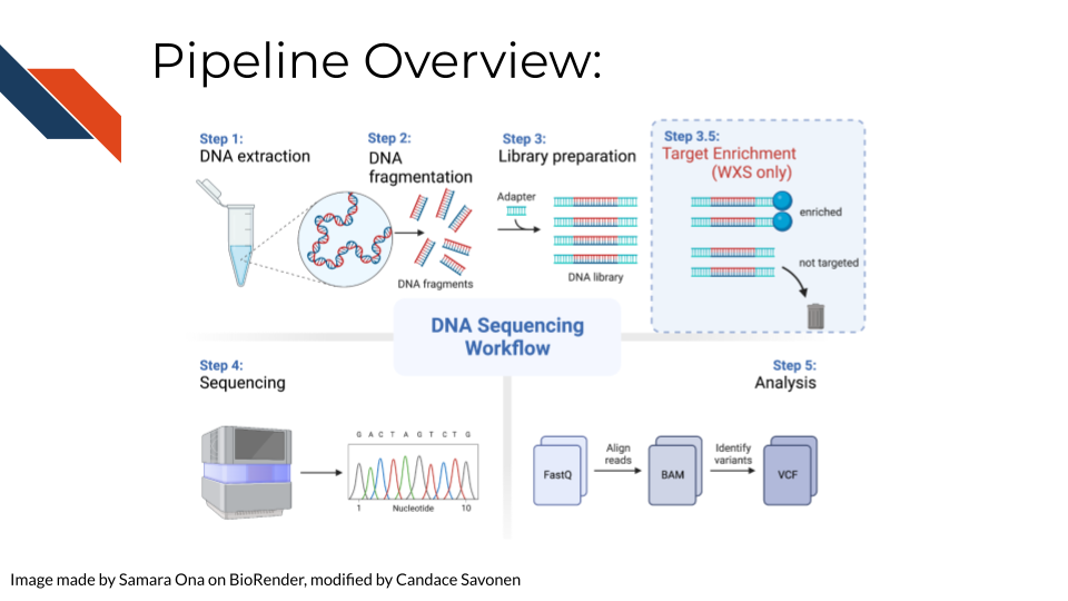In order to create WGS/WXS data, DNA is first extracted from a specific sample type (tissue, blood samples, cells, FFPE blocks, etc.). Either traditional (involving phenol and chloroform) or commercial kits can be used for this first step. Next, the DNA sequencing libraries are prepared. This involves fragmenting the DNA, adding sequencing adapters, and DNA amplification if the input DNA is not of sufficient quantity. Recall that for WXS After sequencing, data is analyzed by converting and aligning reads to generate a BAM file. Many analysis tools will use the BAM file to identify variants, which then generates a VCF file. More information about sequencing and BAM and VCF file generation can be found here in the sequencing data chapter.

10.6 Data Pre-processing

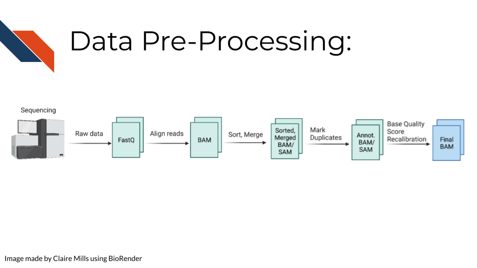Raw sequencing reads are first transformed into a fastq file (more information about fastq files can be found here in the sequencing data chapter in the Quality Controls section. Then the sequencing reads are aligned to a reference genome to create a BAM file. This data is sorted and merged, and PCR duplicates are identified. The confidence that each read was sequenced correctly is reflected in the base quality score. This score must be recalibrated at this step before variants are called. A final BAM file is thus created. This can be used for future analysis steps include variant or mutation identification, which is outlined on the following slide.

10.7 Commonly Used Tools

The following link provides the data analysis pipeline written by researchers in the NCI division of the NIH and provides a helpful overview of the typical steps necessary for WGS analysis.

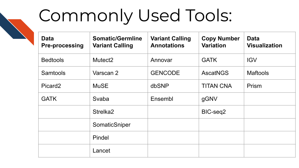
Here are many of the tools and resources used by researchers for analyzing WGS data.

10.8 Data pre-processing tools

In most cases, all of these tools will be used sequentially to prepare the data for downstream mutational and copy number variation (CNV) analysis.

• Bedtools including the bamtofastq function, which is the first step in converting data off the sequencer to a usable format for downstream analysis
• Samtools including tools for converting fastq to BAM files while mapping genes to the genome, duplicate read marking, and sorting reads
• Picard2 including tools to covert fastq to SAM files, filter files, create indices, mark read duplicates, sort files, and merge files
• GATK is a comprehensive set of tools from the Broad Institute for analyzing many types of sequencing data. For pre-processing, the print read function is very beneficial for writing the reads from a BAM or SAM file that pass specific criteria to a new file

10.9 Tools for somatic and germline variant identification

These tools are used to identify either somatic or germline mutations from a sequenced sample. Many researchers will often use a combination of these tools to narrow down only variants that are identified using a combination of these analysis algorithms. All of these mutation calling tools except SvABA can be used on both WGS and WXS data.

• Mutect2 This is a beneficial variant calling tool with functions including using a “panel of normals” (samples provided by the user of many normal controls) to better compare disease samples to normal and filtering functions for samples with orientation bias artifacts (FFPE samples) called F1R2, which is explained in the link above.
• Varscan 2 This is a helpful tool that utilizes a heuristic/statistic approach to variant calling. This means that it detects somatic CNAs (SCNAs) as deviations from the log-ratio of sequence coverage depth within a tumor–normal pair, and then quantify the deviations statistically. This approach is unique because it accounts for differences in read depth between the tumor and normal sample. Varscan 2 can also be used for identifying copy number alterations in tumor-normal pairs.
• MuSE This is a beneficial mutation calling tool when you have both tumor and normal datasets. The Markov Substitution Model for Evolution utilized in this tool models the evolution of the reference allele to the allelic composition of the tumor and normal tissue at each genomic locus.
• SvABA This tool is especially useful for calling insertions and deletions (indels) because it assembles aberrantly aligned sequence reads that reflect indels or structural variants using a custom String Graph Assembler. Indels can be difficult to detect with standard alignment-based variant callers.
• Strelka2 This is a small variant caller designed by Illumina. It is used for identifying germline variants in cohorts of samples and somatic variants in tumor/normal sample pairs.
• SomaticSniper SomaticSniper can be used to identify SNPs in tumor/normal pairs. It calculates the probability that the tumor and normal genotypes are different and reports this probability as a somatic score.
• Pindel Pindel is a tool that uses a pattern growth approach to detect breakpoints of large deletions, medium size insertion/inversion, tandem duplications.
• Lancet This is a newer variant calling tool that uses colored de Bruijn graphs to jointly analyze tumor and normal pairs, offering strong indel detection. More information about the processes used in this variant calling tool can be found here

Researchers may want to create a consensus file based on the mutation calls using multiple tools above. OpenPBTA-analysis shows an open source code example of how you might compare and contrast different SNV caller’s results.

For researchers who prefer GUI based platforms: Gene Pattern has a great set of variant based tutorials. GenePattern is an open software environment providing access to hundreds of tools for the analysis and visualization of genomic data.

10.10 Tools for variant calling annotation

These are beneficial for providing functional meaning to the mutational hits identified above.

• Annovar This is a helpful tool for annotating, filtering, and combining the output data from the above tools. It can be used for gene-based, region-based, or filter-based annotations.
• GENCODE This tool can be used to identify and classify gene features in human and mouse genomes.
• dbSNP This is a resource to look up specific human single nucleotide variations, microsatellites, and small-scale insertions and deletions.
• Ensembl This resource is a genome browser for annotating genes from a wide variety of species.
• pVACtools supports identification of altered peptides from different mechanisms, including point mutations, in-frame and frameshift insertions and deletions, and gene fusions.

10.11 Tools for copy number variation analysis

Similar to the mutation calling tools, many researchers will use several of these tools and investigate the overlapping hits seen with different copy number variant calling algorithms:

• GATK GATK has a variety of tools that can be used to study changes in copy numbers of genes. This link provides a tutorial for how to use the tools.
• AscatNGS These tools (allele-specific copy number analysis of tumors) are specific for WGS copy number variation analysis. They can be used to dissect allele-specific copy numbers of tumors by estimating and adjusting for tumor ploidy and nonaberrant cell admixture.
  
• TitanCNA This tool is used to analyze copy number variation and loss of heterozygosity at the subclonal level for both WGS and WXS data in tumors compared to matched normals. It accounts for mixtures of cell populations and estimates the proportion of cells harboring each event. The Ha lab has developed a snakemake pipeline to more easily use this tool. Ha et al. published a paper describing this tool in detail here
  
• gGNV This is a germline CNV calling tool that can be used on both WGS and WXS data. This tool has booth COHORT and CASE modes. COHORT mode is used when providing a cohort of germline samples where CASE mode is used for individual samples. More details about these modes are described in the link above.
  
• BIC-seq2 This tool is used to detect CNVs with or without control samples. The steps involved in this data processing tool include normalization and CNV detection.

10.12 Tools for data visualization

These tools are often used in parallel to look at regions of the genome, develop plots, and create other relevant figures:

• OpenCRAVAT uses variation data in many popular variant file formats and its outputs are variant annotations and visualizations.
• IGV IGV is an interactive tool used to easily visualize genomic data. It is available as a desktop application, web application, and JavaScript to embed in web pages. This application is very beneficial for visualizing both mutational and CNV data for WGS and WXS. IGV has many tutorials on YouTube that are helpful for using the tool to its full potential.
• Maftools Maftools is an R package that can be used to create informative plots from your WGS data output. It has tools to import both VCF files and ANNOVAR output for data analysis.
• Prism Prism is a widely used tool in scientific research for organizing large datasets, generating plots, and creating readable figures. WGS or WXS data regarding mutations and CNV can be used as input for creating plots with this tool.

10.13 Resources for WGS

Online tutorials:

• Galaxy tutorials
• NCI resources
• Bioinformaticsdotca tutorial

Papers comparing analysis tools:

• (Hwang et al. 2019)
• (Naj et al. 2019)
• (X. He et al. 2020)

References

He, Xiaoyu, Shanyu Chen, Ruilin Li, Xinyin Han, Zhipeng He, Danyang Yuan, Shuying Zhang, Xiaohong Duan, and Beifang Niu. 2020. “Comprehensive Fundamental Somatic Variant Calling and Quality Management Strategies for Human Cancer Genomes.” Briefings in Bioinformatics 22 (3). https://doi.org/10.1093/bib/bbaa083.

Hwang, Kyu-Baek, In-Hee Lee, Honglan Li, Dhong-Geon Won, Carles Hernandez-Ferrer, Jose Alberto Negron, and Sek Won Kong. 2019. “Comparative Analysis of Whole-Genome Sequencing Pipelines to Minimize False Negative Findings.” Scientific Reports 9 (1). https://doi.org/10.1038/s41598-019-39108-2.

Naj, Adam C., Honghuang Lin, Badri N. Vardarajan, Simon White, Daniel Lancour, Yiyi Ma, Michael Schmidt, et al. 2019. “Quality Control and Integration of Genotypes from Two Calling Pipelines for Whole Genome Sequence Data in the Alzheimers Disease Sequencing Project.” Genomics 111 (4): 808–18. https://doi.org/10.1016/j.ygeno.2018.05.004.

---

All illustrations CC-BY.
All other materials CC-BY unless noted otherwise.