
Chapter 5 Data Wrangling with Tidy Data, Part 2
Today, we will continue learning about common functions from the Tidyverse that is useful for Tidy data manipulations.
5.1 Modifying and creating new columns in dataframes
The mutate() function takes in the following arguments: the first argument is the dataframe of interest, and the second argument is a new or existing data variable that is defined in terms of other data variables.
We create a new column olderAge that is 10 years older than the original Age column.
## [1] 60 36 72 30 30 64 63 56 72 53## [1] 70 46 82 40 40 74 73 66 82 63Here, we used an operation on a column of metadata. Here’s another example with a function:
##  [1] 4.634012 4.638653 4.032101 5.503031 3.713696 3.972693 3.235727 4.135042
## [9] 9.017365 3.940167## [1] 1.533423 1.534424 1.394288 1.705299 1.312028 1.379444 1.174254 1.419498
## [9] 2.199152 1.3712235.2 Merging two dataframes together
Suppose we have the following dataframes:
expression
| ModelID | PIK3CA_Exp | log_PIK3CA_Exp |
|---|---|---|
| “ACH-001113” | 5.138733 | 1.636806 |
| “ACH-001289” | 3.184280 | 1.158226 |
| “ACH-001339” | 3.165108 | 1.152187 |
metadata
| ModelID | OncotreeLineage | Age |
|---|---|---|
| “ACH-001113” | “Lung” | 69 |
| “ACH-001289” | “CNS/Brain” | NA |
| “ACH-001339” | “Skin” | 14 |
Suppose that I want to compare the relationship between OncotreeLineage and PIK3CA_Exp, but they are columns in different dataframes. We want a new dataframe that looks like this:
| ModelID | PIK3CA_Exp | log_PIK3CA_Exp | OncotreeLineage | Age |
|---|---|---|---|---|
| “ACH-001113” | 5.138733 | 1.636806 | “Lung” | 69 |
| “ACH-001289” | 3.184280 | 1.158226 | “CNS/Brain” | NA |
| “ACH-001339” | 3.165108 | 1.152187 | “Skin” | 14 |
We see that in both dataframes, the rows (observations) represent cell lines with a common column ModelID, so let’s merge these two dataframes together, using full_join():
The number of rows and columns of metadata:
## [1] 1864 30The number of rows and columns of expression:
## [1] 1450 536The number of rows and columns of merged:
## [1] 1864 565We see that the number of columns in merged combines the number of columns in metadata and expression, while the number of rows in merged is the larger of the number of rows in metadata and expression : full_join() keeps all observations common to both dataframes based on the common column defined via the by argument.
Therefore, we expect to see NA values in merged, as there are some cell lines that are not in expression dataframe.
There are variations of this function depending on your application:
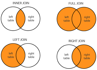
Given xxx_join(x, y, by = "common_col"),
full_join()keeps all observations.left_join()keeps all observations inx.right_join()keeps all observations iny.inner_join()keeps observations common to bothxandy.
5.3 Grouping and summarizing dataframes
In a dataset, there may be multiple levels of observations, and which level of observation we examine depends on our scientific question. For instance, in metadata, the observation is cell lines. However, perhaps we want to understand properties of metadata in which the observation is the cancer type, OncotreeLineage. Suppose we want the mean age of each cancer type, and the number of cell lines that we have for each cancer type.
This is a scenario in which the desired rows are described by a column, OncotreeLineage, and the columns, such as mean age, need to be summarized from other columns.
As an example, this dataframe is transformed from:
| ModelID | OncotreeLineage | Age |
|---|---|---|
| “ACH-001113” | “Lung” | 69 |
| “ACH-001289” | “Lung” | 23 |
| “ACH-001339” | “Skin” | 14 |
| “ACH-002342” | “Brain” | 23 |
| “ACH-004854” | “Brain” | 56 |
| “ACH-002921” | “Brain” | 67 |
into:
| OncotreeLineage | MeanAge | Count |
|---|---|---|
| “Lung” | 46 | 2 |
| “Skin” | 14 | 1 |
| “Brain” | 48.67 | 3 |
We use the functions group_by() and summarise() :
metadata_by_type = metadata |>
                   group_by(OncotreeLineage) |>
                   summarise(MeanAge = mean(Age, rm.na=TRUE), Count = n())
Or, without pipes:
metadata_by_type_temp = group_by(metadata, OncotreeLineage)
metadata_by_type = summarise(metadata_by_type_temp, MeanAge = mean(Age, rm.na=TRUE), Count = n())
The group_by() function returns the identical input dataframe but remembers which variable(s) have been marked as grouped:
## # A tibble: 6 × 30
## # Groups:   OncotreeLineage [3]
##   ModelID    PatientID CellLineName StrippedCellLineName   Age SourceType
##   <chr>      <chr>     <chr>        <chr>                <dbl> <chr>
## 1 ACH-000001 PT-gj46wT NIH:OVCAR-3  NIHOVCAR3               60 Commercial
## 2 ACH-000002 PT-5qa3uk HL-60        HL60                    36 Commercial
## 3 ACH-000003 PT-puKIyc CACO2        CACO2                   72 Commercial
## 4 ACH-000004 PT-q4K2cp HEL          HEL                     30 Commercial
## 5 ACH-000005 PT-q4K2cp HEL 92.1.7   HEL9217                 30 Commercial
## 6 ACH-000006 PT-ej13Dz MONO-MAC-6   MONOMAC6                64 Commercial
## # ℹ 24 more variables: SangerModelID <chr>, RRID <chr>, DepmapModelType <chr>,
## #   AgeCategory <chr>, GrowthPattern <chr>, LegacyMolecularSubtype <chr>,
## #   PrimaryOrMetastasis <chr>, SampleCollectionSite <chr>, Sex <chr>,
## #   SourceDetail <chr>, LegacySubSubtype <chr>, CatalogNumber <chr>,
## #   CCLEName <chr>, COSMICID <dbl>, PublicComments <chr>,
## #   WTSIMasterCellID <dbl>, EngineeredModel <chr>, TreatmentStatus <chr>,
## #   OnboardedMedia <chr>, PlateCoating <chr>, OncotreeCode <chr>, …
The summarise() returns one row for each combination of grouping variables, and one column for each of the summary statistics that you have specified.
Functions you can use for summarise() must take in a vector and return a simple data type, such as any of our summary statistics functions: mean(), median(), min(), max(), etc.
The exception is n(), which returns the number of entries for each grouping variable’s value.
You can combine group_by() with other functions. See this guide.
5.4 Exercises
You can find exercises and solutions on Posit Cloud, or on GitHub.