
Chapter 4 Data Wrangling with Tidy Data, Part 1
4.1 Explicit vs. implicit subsetting
Suppose you are given this vector:
Here are two scenarios of subsetting:
Explicit subsetting: Suppose someone approaches you a length 10 vector of people’s ages, and say that they want to subset to the 1st, 3rd, and 9th elements.
Implicit subsetting: Suppose someone approaches you a length 10 vector of people’s ages, and say that they want to subset to elements greater than 50.
We already know how to subset explicitly:
## [1] 89 64 30But for implicit subsetting, we don’t know off the top of our head which elements have a value greater than 50. If this vector was really big, it wouldn’t make sense for us to manually figure this out. Luckily, we already have the tools we need to subset vectors implicitly.
Recall that our comparison operators can be applied for vectors, such as:
## [1] TRUE TRUE TRUE TRUE TRUE TRUE TRUE TRUE FALSE FALSEThis vector of TRUE and FALSE values can be used as a logical indexing vector to help us subset implicitly!
## [1] 89 70 64 90 66 71 55 60Subset a vector implicitly, in 3 steps:
- Come up with a criteria for subsetting: “I want to subset to values greater than 50”.
- We can use a comparison operator to create a logical indexing vector that fits this criteria.
## [1] TRUE TRUE TRUE TRUE TRUE TRUE TRUE TRUE FALSE FALSE- Use this logical indexing vector to subset.
## [1] 89 70 64 90 66 71 55 60Alternatively,
## [1] 89 70 64 90 66 71 55 60And you are done.
For most of our subsetting tasks on vectors (and dataframes below), we will be encouraging implicit subsetting. The power of implicit subsetting is that you don’t need to know what your vector contains to do something with it! This technique is related to abstraction in programming mentioned in the first lesson: by using expressions to find the specific value you are interested instead of hard-coding the value explicitly, it generalizes your code to handle a wider variety of situations.
One more example:
Let’s subset staff so it doesn’t have “chris” in it.
Use an appropriate comparison operator:
## [1] FALSE TRUE TRUEThen, use the resulting value as a logical indexing vector:
## [1] "sonu" "sean"We stored the subsetted result as a variable answer.
Let’s take this idea of implicit subsetting to Dataframes.
4.2 Data Science workflow
From our first two lessons, we are now equipped with enough fundamental programming skills to apply it to various steps in the data science workflow, which is a natural cycle that occurs in data analysis.

For the rest of the course, we focus on Transform and Visualize with the assumption that our data is in a nice, “Tidy format”. First, we need to understand what it means for a data to be “Tidy”.
4.3 Tidy Data
Here, we describe a standard of organizing data. It is important to have standards, as it facilitates a consistent way of thinking about data organization and building tools (functions) that make use of that standard. The principles of tidy data, developed by Hadley Wickham:
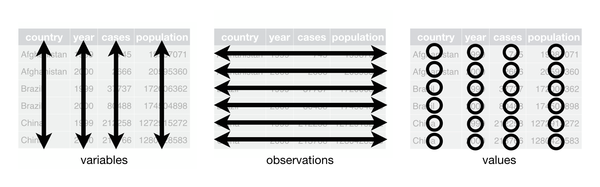
Each variable must have its own column.
Each observation must have its own row.
Each value must have its own cell.
If you want to be technical about what variables and observations are, Hadley Wickham describes:
A variable contains all values that measure the same underlying attribute (like height, temperature, duration) across units. An observation contains all values measured on the same unit (like a person, or a day, or a race) across attributes.
4.4 Examples and counter-examples of Tidy Data:
Consider the following three datasets, which all contain the exact same information:
## # A tibble: 6 × 4
##   country      year  cases population
##   <chr>       <dbl>  <dbl>      <dbl>
## 1 Afghanistan  1999    745   19987071
## 2 Afghanistan  2000   2666   20595360
## 3 Brazil       1999  37737  172006362
## 4 Brazil       2000  80488  174504898
## 5 China        1999 212258 1272915272
## 6 China        2000 213766 1280428583
This table1 satisfies the the definition of Tidy Data. The observation is a country’s year, and the variables are attributes of each country’s year.
## # A tibble: 6 × 4
##   country      year type           count
##   <chr>       <dbl> <chr>          <dbl>
## 1 Afghanistan  1999 cases            745
## 2 Afghanistan  1999 population  19987071
## 3 Afghanistan  2000 cases           2666
## 4 Afghanistan  2000 population  20595360
## 5 Brazil       1999 cases          37737
## 6 Brazil       1999 population 172006362
Something is strange able table2. The observation is still a country’s year, but “type” and “count” are not clear attributes of each country’s year.
## # A tibble: 6 × 3
##   country      year rate
##   <chr>       <dbl> <chr>
## 1 Afghanistan  1999 745/19987071
## 2 Afghanistan  2000 2666/20595360
## 3 Brazil       1999 37737/172006362
## 4 Brazil       2000 80488/174504898
## 5 China        1999 212258/1272915272
## 6 China        2000 213766/1280428583
In table3, we have multiple values for each cell under the “rate” column.
4.5 Our working Tidy Data: DepMap Project
The Dependency Map project is a multi-omics profiling of cancer cell lines combined with functional assays such as CRISPR and drug sensitivity to help identify cancer vulnerabilities and drug targets. Here are some of the data that we have public access. We have been looking at the metadata since last session.
Metadata
Somatic mutations
Gene expression
Drug sensitivity
CRISPR knockout
and more…
Let’s see how these datasets fit the definition of Tidy data:
| Dataframe | The observation is | Some variables are | Some values are |
|---|---|---|---|
| metadata | Cell line | ModelID, Age, OncotreeLineage | “ACH-000001”, 60, “Myeloid” |
| expression | Cell line | KRAS_Exp | 2.4, .3 |
| mutation | Cell line | KRAS_Mut | TRUE, FALSE |
4.6 Transform: “What do you want to do with this dataframe”?
Until now, we haven’t focused too much on how we organize our scientific ideas to interact with what we can do with code. Let’s pivot to write our code driven by our scientific curiosity. After we are sure that we are working with Tidy data, we can ponder how we want to transform our data that satisfies our scientific question. We will look at several ways we can transform Tidy data, starting with subsetting columns and rows.
Here’s a starting prompt:
In the
metadatadataframe, which rows would you filter for and columns would you select that relate to a scientific question?
We should use the implicit subsetting mindset here: ie. “I want to filter for rows such that the Subtype is breast cancer and look at the Age and Sex.” and not “I want to filter for rows 20-50 and select columns 2 and 8”.
Notice that when we filter for rows in an implicit way, we often formulate our criteria about the columns.
(This is because we are guaranteed to have column names in dataframes, but not usually row names. Some dataframes have row names, but because the data types are not guaranteed to have the same data type across rows, it makes describing by row properties difficult.)
Let’s convert our implicit subsetting criteria into code!
metadata_filtered = filter(metadata, OncotreeLineage == "Breast")
breast_metadata = select(metadata_filtered, ModelID, Age, Sex)

head(breast_metadata)
## ModelID Age Sex
## 1 ACH-000017 43 Female
## 2 ACH-000019 69 Female
## 3 ACH-000028 69 Female
## 4 ACH-000044 47 Female
## 5 ACH-000097 63 Female
## 6 ACH-000111 41 FemaleHere, filter() and select() are functions from the tidyverse package, which we have to install and load in via library(tidyverse) before using these functions.
4.6.1 Filter rows
Let’s carefully a look what how the R Console is interpreting the filter() function:
We evaluate the expression right of
=.The first argument of
filter()is a dataframe, which we givemetadata.The second argument is strange: the expression we give it looks like a logical indexing vector built from a comparison operator, but the variable
OncotreeLineagedoes not exist in our environment! Rather,OncotreeLineageis a column frommetadata, and we are referring to it as a data variable in the context of the dataframemetadata. So, we make a comparison operation on the columnOncotreeLineagefrommetadataand its resulting logical indexing vector is the input to the second argument.How do we know when a variable being used is a variable from the environment, or a data variable from a dataframe? It’s not clear cut, but here’s a rule of thumb: most functions from the
tidyversepackage allows you to use data variables to refer to columns of a dataframe. We refer to documentation when we are not sure.This encourages more readable code at the expense of consistency of referring to variables in the environment. The authors of this package describes this trade-off.
Putting it together,
filter()takes in a dataframe, and an logical indexing vector described by data variables as arguments, and returns a data frame with rows that match condition described by the logical indexing vector.Store this in
metadata_filteredvariable.
4.6.2 Select columns
Let’s carefully a look what how the R Console is interpreting the select() function:
We evaluate the expression right of
=.The first argument of
filter()is a dataframe, which we givemetadata.The second and third arguments are data variables referring the columns of
metadata.- For certain functions like
filter(), there is no limit on the number of arguments you provide. You can keep adding data variables to select for more column names.
- For certain functions like
Putting it together,
select()takes in a dataframe, and as many data variables you like to select columns, and returns a dataframe with the columns you described by data variables.Store this in
breast_metadatavariable.
4.7 Summary Statistics
Now that your dataframe has be transformed based on your scientific question, you can start doing some analysis on it! A common data science task is to examine summary statistics of a dataset, which summarizes the observations of a variable in a numeric summary.
If the columns of interest are numeric, then you can try functions such as mean(), median(), mode(), or summary() to get summary statistics of the column. If the columns of interest is character or logical, then you can try the table() function.
All of these functions take in a vector as input and not a dataframe, so you have to access the column as a vector via the $ operation.
## [1] 50.96104##
## Female Unknown
## 91 1When computing the mean value of the Age column from breast_metadata, we add an additional option of na.rm = TRUE because some of the column contain missing values. This will remove the missing values before computing the mean value.
4.8 Pipes
Often, in data analysis, we want to transform our dataframe in multiple steps via different functions. This leads to nested function calls, like this:
This is a bit hard to read. A computer doesn’t care how difficult it is to read this line of code, but there is a lot of instructions going on in one line of code. This multi-step function composition will lead to an unreadable pattern such as:
result = function3(function2(function1(dataframe, df_col4, df_col2), arg2), df_col5, arg1)To untangle this, you have to look into the middle of this code, and slowly step out of it.
To make this more readable, programmers came up with an alternative syntax for function composition via the pipe metaphor. The ideas is that we push data through a chain of connected pipes, in which the output of a pipe becomes the input of the subsequent pipe.
Instead of a syntax like result2 = function3(function2(function1(dataframe))),
we linearize it with the |> symbol: result2 = dataframe |> function1 |> function2 |> function3.
In the previous example,
result = dataframe %>% function1(df_col4, df_col2) |>
         function2(arg2) |>
         function3(df_col5, arg1)
This looks much easier to read. Notice that we have broken up one expression in to three lines of code for readability. If a line of code is incomplete (the first line of code is piping to somewhere unfinished), the R will treat the next line of code as part of the current line of code.
Try to rewrite the select() and filter() function composition example above using the pipe metaphor and syntax.
4.9 Exercises
You can find exercises and solutions on Posit Cloud, or on GitHub.