
Chapter 4 Data Wrangling, Part 2
We will continue to learn about data analysis with Dataframes. Let’s load our three Dataframes from the Depmap project in again:
import pandas as pd
import numpy as np

metadata = pd.read_csv("classroom_data/metadata.csv")
mutation = pd.read_csv("classroom_data/mutation.csv")
expression = pd.read_csv("classroom_data/expression.csv")
4.1 Creating new columns
Often, we want to perform some kind of transformation on our data’s columns: perhaps you want to add the values of columns together, or perhaps you want to represent your column in a different scale.
To create a new column, you simply modify it as if it exists using the bracket operation [ ], and the column will be created:
metadata['AgePlusTen'] = metadata['Age'] + 10
expression['KRAS_NRAS_exp'] = expression['KRAS_Exp'] + expression['NRAS_Exp']
expression['log_PIK3CA_Exp'] = np.log(expression['PIK3CA_Exp'])
where np.log(x) is a function imported from the module NumPy that takes in a numeric and returns the log-transformed value.
Note: you cannot create a new column referring to the attribute of the Dataframe, such as: expression.KRAS_Exp_log = np.log(expression.KRAS_Exp).
4.2 Merging two Dataframes together
Suppose we have the following Dataframes:
expression
| ModelID | PIK3CA_Exp | log_PIK3CA_Exp |
|---|---|---|
| “ACH-001113” | 5.138733 | 1.636806 |
| “ACH-001289” | 3.184280 | 1.158226 |
| “ACH-001339” | 3.165108 | 1.152187 |
metadata
| ModelID | OncotreeLineage | Age |
|---|---|---|
| “ACH-001113” | “Lung” | 69 |
| “ACH-001289” | “CNS/Brain” | NaN |
| “ACH-001339” | “Skin” | 14 |
Suppose that I want to compare the relationship between OncotreeLineage and PIK3CA_Exp, but they are columns in different Dataframes. We want a new Dataframe that looks like this:
| ModelID | PIK3CA_Exp | log_PIK3CA_Exp | OncotreeLineage | Age |
|---|---|---|---|---|
| “ACH-001113” | 5.138733 | 1.636806 | “Lung” | 69 |
| “ACH-001289” | 3.184280 | 1.158226 | “CNS/Brain” | NaN |
| “ACH-001339” | 3.165108 | 1.152187 | “Skin” | 14 |
We see that in both dataframes,
the rows (observations) represent cell lines.
there is a common column
ModelID, with shared values between the two dataframes that can faciltate the merging process. We call this an index.
We will use the method .merge() for Dataframes. It takes a Dataframe to merge with as the required input argument. The method looks for a common index column between the two dataframes and merge based on that index.
It’s usually better to specify what that index column to avoid ambiguity, using the on optional argument:
If the index column for the two Dataframes are named differently, you can specify the column name for each Dataframe:
One of the most import checks you should do when merging dataframes is to look at the number of rows and columns before and after merging to see whether it makes sense or not:
The number of rows and columns of metadata:
## (1864, 31)The number of rows and columns of expression:
## (1450, 538)The number of rows and columns of merged:
## (1450, 568)We see that the number of columns in merged combines the number of columns in metadata and expression, while the number of rows in merged is the smaller of the number of rows in metadata and expression: it only keeps rows that are found in both Dataframe’s index columns. This kind of join is called “inner join”, because in the Venn Diagram of elements common in both index column, we keep the inner overlap:
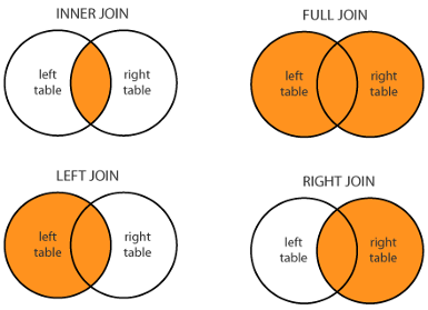
You can specifiy the join style by changing the optional input argument how.
how = "outer"keeps all observations - also known as a “full join”how = "left"keeps all observations in the left Dataframe.how = "right"keeps all observations in the right Dataframe.how = "inner"keeps observations common to both Dataframe. This is the default value ofhow.
4.3 Grouping and summarizing Dataframes
In a dataset, there may be groups of observations that we want to understand, such as case vs. control, or comparing different cancer subtypes. For example, in metadata, the observation is cell lines, and perhaps we want to group cell lines into their respective cancer type, OncotreeLineage, and look at the mean age for each cancer type.
We want to take metadata:
| ModelID | OncotreeLineage | Age |
|---|---|---|
| “ACH-001113” | “Lung” | 69 |
| “ACH-001289” | “Lung” | 23 |
| “ACH-001339” | “Skin” | 14 |
| “ACH-002342” | “Brain” | 23 |
| “ACH-004854” | “Brain” | 56 |
| “ACH-002921” | “Brain” | 67 |
into:
| OncotreeLineage | MeanAge |
|---|---|
| “Lung” | 46 |
| “Skin” | 14 |
| “Brain” | 48.67 |
To get there, we need to:
Group the data based on some criteria, elements of
OncotreeLineageSummarize each group via a summary statistic performed on a column, such as
Age.
We use the methods .group_by(x) and .mean().
## OncotreeLineage
## Adrenal Gland                55.000000
## Ampulla of Vater             65.500000
## Biliary Tract                58.450000
## Bladder/Urinary Tract        65.166667
## Bone                         20.854545
## Bowel                        58.611111
## Breast                       50.961039
## CNS/Brain                    43.849057
## Cervix                       47.136364
## Esophagus/Stomach            57.855556
## Eye                          51.100000
## Fibroblast                   38.194444
## Head and Neck                60.149254
## Kidney                       46.193548
## Liver                        43.928571
## Lung                         55.444444
## Lymphoid                     38.916667
## Myeloid                      38.810811
## Normal                       52.370370
## Other                        46.000000
## Ovary/Fallopian Tube         51.980769
## Pancreas                     60.226415
## Peripheral Nervous System     5.480000
## Pleura                       61.000000
## Prostate                     61.666667
## Skin                         49.033708
## Soft Tissue                  27.500000
## Testis                       25.000000
## Thyroid                      63.235294
## Uterus                       62.060606
## Vulva/Vagina                 75.400000
## Name: Age, dtype: float64
Here’s what’s going on:
We use the Dataframe method
.group_by(x)and specify the column we want to group by. The output of this method is a Grouped Dataframe object. It still contains all the information of themetadataDataframe, but it makes a note that it’s been grouped.We subset to the column
Age. The grouping information still persists (This is a Grouped Series object).We use the method
.mean()to calculate the mean value ofAgewithin each group defined byOncotreeLineage.
Alternatively, this could have been done in a chain of methods:
## OncotreeLineage
## Adrenal Gland                55.000000
## Ampulla of Vater             65.500000
## Biliary Tract                58.450000
## Bladder/Urinary Tract        65.166667
## Bone                         20.854545
## Bowel                        58.611111
## Breast                       50.961039
## CNS/Brain                    43.849057
## Cervix                       47.136364
## Esophagus/Stomach            57.855556
## Eye                          51.100000
## Fibroblast                   38.194444
## Head and Neck                60.149254
## Kidney                       46.193548
## Liver                        43.928571
## Lung                         55.444444
## Lymphoid                     38.916667
## Myeloid                      38.810811
## Normal                       52.370370
## Other                        46.000000
## Ovary/Fallopian Tube         51.980769
## Pancreas                     60.226415
## Peripheral Nervous System     5.480000
## Pleura                       61.000000
## Prostate                     61.666667
## Skin                         49.033708
## Soft Tissue                  27.500000
## Testis                       25.000000
## Thyroid                      63.235294
## Uterus                       62.060606
## Vulva/Vagina                 75.400000
## Name: Age, dtype: float64
Once a Dataframe has been grouped and a column is selected, all the summary statistics methods you learned from last week, such as .mean(), .median(), .max(), can be used. One new summary statistics method that is useful for this grouping and summarizing analysis is .count() which tells you how many entries are counted within each group.
4.3.1 Optional: Multiple grouping, Multiple columns, Multiple summary statistics
Sometimes, when performing grouping and summary analysis, you want to operate on multiple columns simultaneously.
For example, you may want to group by a combination of OncotreeLineage and AgeCategory, such as “Lung” and “Adult” as one grouping. You can do so like this:
metadata_grouped = metadata.groupby(["OncotreeLineage", "AgeCategory"])
metadata_grouped['Age'].mean()
## OncotreeLineage AgeCategory
## Adrenal Gland Adult 55.000000
## Ampulla of Vater Adult 65.500000
## Unknown NaN
## Biliary Tract Adult 58.450000
## Unknown NaN
## ...
## Thyroid Unknown NaN
## Uterus Adult 62.060606
## Fetus NaN
## Unknown NaN
## Vulva/Vagina Adult 75.400000
## Name: Age, Length: 72, dtype: float64You can also summarize on multiple columns simultaneously. For each column, you have to specify what summary statistic functions you want to use. This can be specified via the .agg(x) method on a Grouped Dataframe.
For example, coming back to our age case-control Dataframe,
df = pd.DataFrame(data={'status': ["treated", "untreated", "untreated", "discharged", "treated"],
                            'age_case': [25, 43, 21, 65, 7],
                            'age_control': [49, 20, 32, 25, 32]})

df
## status age_case age_control
## 0 treated 25 49
## 1 untreated 43 20
## 2 untreated 21 32
## 3 discharged 65 25
## 4 treated 7 32We group by status and summarize age_case and age_control with a few summary statistics each:
##            age_case age_control
##                mean         min max  mean
## status
## discharged     65.0          25  25  25.0
## treated        16.0          32  49  40.5
## untreated      32.0          20  32  26.0
The input argument to the .agg(x) method is called a Dictionary, which let’s you structure information in a paired relationship. You can learn more about dictionaries here.
4.4 Exercises
Exercise for week 4 can be found here.