
Chapter 11 Part 2. Summarizing with Statistics
Now that we have the dataset loaded, let’s explore the data in more depth.
First, we should remove those samples that don’t have soil testing data yet. We could keep them in the dataset, but removing them at this stage will make the analysis a little cleaner. In this case, as we know the reason the data are missing (and that reason will not skew our analysis), we can safely remove these samples. This will not be the case for every data analysis.
We can remove the unanalyzed samples using the drop_na() function from the tidyverse package. The tidyverse package is a collection of code that makes organizing data tables (also known as data wrangling) easy in R. The drop_na function removes any rows from a table that contains NA for a particular column. This command follows the code structure:
dataset_new_name <- dataset_object_name %>% drop_na(column_name)
The %>% is called a pipe and it tells R that the commands after it should all be applied to the object in front of it. (In this case, we can filter out all samples missing a value for “As_EPA3051” as a proxy for samples without soil testing data.)
The following code block opens the tidyverse package, then tells R to filter out all samples missing a value for “As_EPA3051” (as a proxy for samples without soil testing data) from the soil.values object, and finally to save the new, filtered dataset as an object called soil.values.clean.
#install.packages('tidyverse') if you haven't already installed the tidyverse!

library(tidyverse)

soil.values.clean <- soil.values %>% drop_na(As_EPA3051)
Great! Now let’s calculate some basic statistics. For example, we might want to know what the mean (average) arsenic concentration is for all the soil samples. We can use a combination of two functions: pull() and mean(). pull() lets you extract a column from your table for statistical analysis, while mean() calculates the average value for the extracted column.
This command follows the code structure:
object_name %>% pull(column_name) %>% mean()
For this chunk of code, R will calculate the mean for the AS_EPA3051 values in the soil.values.clean dataset. Because we have not used the <- to save the mean in a new object, R will simply display the mean.
## [1] 5.10875We can run similar commands to calculate the standard deviation (sd),
minimum (min), and maximum (max) for the soil arsenic values.
## [1] 5.606926## [1] 0## [1] 27.3The soil testing dataset contains samples from multiple geographic regions, so maybe it’s more meaningful to find out what the average arsenic values are for each region. However, first we need to grab a new dataset from the BioDIGSData package that tells us the geographic regions of each sample.
Let’s open BioDIGS_metadata, save it as soil.meta, and look at it.
The metadata (or, data about the samples) contains information stored as 7 different variables. We can see that this dataset contains a variable called site_id that matches a column in the soil.values and soil.values.clean datasets. This is important! Using this variable, we can combine the soil.values.clean and soil.meta into a single dataset.
The command for combining the datasets follows the code structure:
combined_dataset_name <- first_dataset %>% inner_join(second_dataset, by = column_name_in_common)
The inner_join command tells R to combine the first_dataset and the second_dataset based on matching information in the column_name_in_column. It also only keeps those rows that are found in both datasets. Finally, the <- tells R to save this combined dataset as a new object.
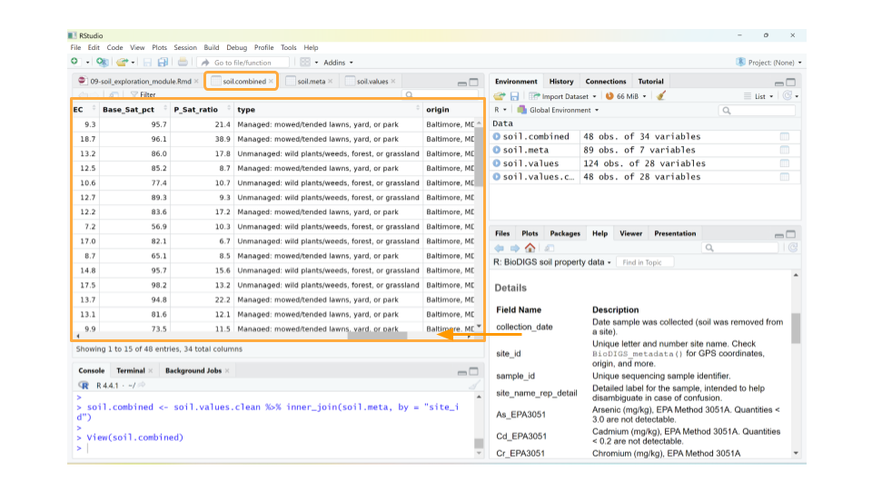
When you scroll through the soil.combined dataset, you now see the metadata columns after all the soil characteristics. In particular, there’s a column called origin which gives the town or city location for each sample. Many of the samples from the pilot study came from 5 places in Maryland: Baltimore, Derwood, Boyds, Germantown, and Bethesda.
Let’s look at the average arsenic content of the soil for each of these locations! We have to do a little bit of clever coding trickery for this using the group_by and summarize functions.
First, we tell R to split our dataset up by a particular column (in this case, origin) using the group_by function, then we tell R to summarize the mean arsenic concentration for each group.
When using the summarize function, we tell R to make a new table (technically, a tibble in R) that contains two columns: the column used to group the data and the statistical measure we calculated for each group.
This command follows the code structure:
dataset %>% group_by(column_name) %>% summarize(mean(column_name))
## # A tibble: 5 × 2
##   origin         `mean(As_EPA3051)`
##   <chr>                       <dbl>
## 1 Baltimore, MD                5.56
## 2 Bethesda, MD                 3.46
## 3 Boyds, MD                    6.94
## 4 Derwood, MD                  4.26
## 5 Germantown, MD               4.30
Now we know that the mean arsenic concentration might be different for each region of origin.
QUESTIONS:
All the samples in the initial pilot study were collected from public park land. Some parks were located in suburban and rural areas, while others were collected from urban parks. Why might soil arsenic concentration be different for rural parks than for urban parks?
What is the mean iron concentration for samples in this dataset? What about the standard deviation, minimum value, and maximum value?
Calculate the mean iron concentration by region of origin. Which region has the highest mean iron concentration? What about the lowest?
Let’s say we’re interested in looking at mean concentration for any element that was determined using EPA Method 3051. Given that there are 8 of these measures in the soil.combined dataset, it would be time consuming to run our code from above that calculates overall mean for each individual measure.
We can add two arguments to our summarize statement to calculate statistical measures for multiple columns at once: the across argument, which tells R to apply the summarize command to multiple columns; and the ends_with parameter, which tells R which columns should be included in the statistical calculation.
We are using ends_with because for this question, all the columns that we’re interested in end with the string ‘EPA3051’.
This command follows the code structure:
dataset %>% group_by(column_name) %>% summarize(across(ends_with(common_column_name_ending), mean))
## # A tibble: 5 × 8
##   origin       As_EPA3051 Cd_EPA3051 Cr_EPA3051 Cu_EPA3051 Ni_EPA3051 Pb_EPA3051
##   <chr>             <dbl>      <dbl>      <dbl>      <dbl>      <dbl>      <dbl>
## 1 Baltimore, …       5.56     0.359        34.5       35.0       17.4       67.2
## 2 Bethesda, MD       3.46     0.375        67.5       17.0       26.6       41.8
## 3 Boyds, MD          6.94     0.0525       16.8       16.8       12.9       31.6
## 4 Derwood, MD        4.26     0.335        39.5       31.3       35.1       42.1
## 5 Germantown,…       4.30     0.602        19.9       23.3       17.7       38.2
## # ℹ 1 more variable: Zn_EPA3051 <dbl>
This is a much more efficient way to calculate statistics.
QUESTIONS:
Calculate the maximum values for concentrations that were determined using EPA Method 3051. (HINT: change the function you call in the
summarizestatement.) Which of these metals has the maximum concentration you see, and in which region is it found?Calculate both the mean and maximum values for concentrations that were determined using the Mehlich3 test. (HINT: change the terms in the the part of the code that uses
ends_with, as well as the function you call in thesummarizestatement.) Which of these metals has the highest average and maximum concentrations, and in which region are they found?