Introduction to Bioconductor

Understanding S4 Objects

Learning Objectives

• Explain the Bioconductor Project
• Explain the basic structure of Bioconductor S4 objects
• Explain and Utilize SummarizedExperiment objects using the tidySummarizedExperiment package

What is Bioconductor?

• An open-source software project since 2001 for ’omics analyses
• A repository of > 3,500 curated, inter-operable R packages
• A community of developers and users
  • Support site
  • Developer mailing list
  • Zulip chat
  • YouTube channel
  • Annual conferences in North America, Europe and Asia
  • Working groups

Data in bioinformatics is often complex and doesn’t fit into a single data frame.
To deal with this, developers define specialized data containers (termed classes) that match the properties of the data they need to handle.

This aspect is central to the Bioconductor¹ project which uses the same core data infrastructure across packages. This certainly contributed to Bioconductor’s success. Bioconductor package developers are advised to make use of existing infrastructure to provide coherence, interoperability, and stability to the project as a whole.

S4 Bioconductor Objects

At the heart of Bioconductor are the S4 Objects. You can think of these data structures as ways to package together:

• Assay Data, such as an RNAseq count matrix
• Metadata (data about the experiment), including Experimental Design

Part of why Bioconductor works is this data packaging. We can write functions to act on the data in these S4 Objects as part of a processing workflow. As long as we output a Bioconductor S4 object, our routines can work as part of a pipeline. These routines are called methods(), and may come from a variety of packages.

What is a method?

You may have heard of functions and methods - what is the difference?

A working definition of a method is that it is a function that works on a particular object type, such as the SummarizedExperiment type we’re going to investigate in a little bit.

Method is a little bit more specific than a function.

You can think of the Bioconductor S4 objects as taking the place of data.frames in dplyr pipelines - they are the common format that all of the Bioconductor methods work on. They allow Bioconductor methods to be interoperable - we can mix and match methods from various packages to customize our analysis.

Case Study: RNAseq Experiments

Bulk RNAseq experiments are meant to distinguish expression differences between samples or groups of samples.

Please see the concepts section for more in depth details of the processing of RNA-seq experiments.

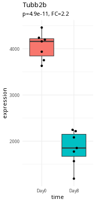
Here is an example of a large expression difference (Tubb2a).

Here is an example of a questionable expression difference (myl7).

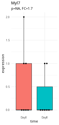
Take a second and think about what makes Tubb2a a better candidate than myl7.

What are we trying to accomplish?

In RNAseq, we are interested in assessing expression differences between samples at either the gene or transcript level. The starting data for this is typically a matrix of counts for thousands of genes and many samples.

In order to do see if there are expression differences, we need phenotype information about the samples in our experiment. Specifically, we need to have information about:

• conditions (infection, time)
• possible confounders (gender)

Experimental Design of RNAseq Experiments

When we design our RNAseq experiment, we want to be able to:

• Number and type of replicates
• Avoiding confounding
• Addressing batch effects

The important thing to note is that if you’re unsure about the experimental design, contact your Bioinformatics Core. They can help you design the experiment based on what samples you have.

Please see the experimental design section for more in depth details.

SummarizedExperiment

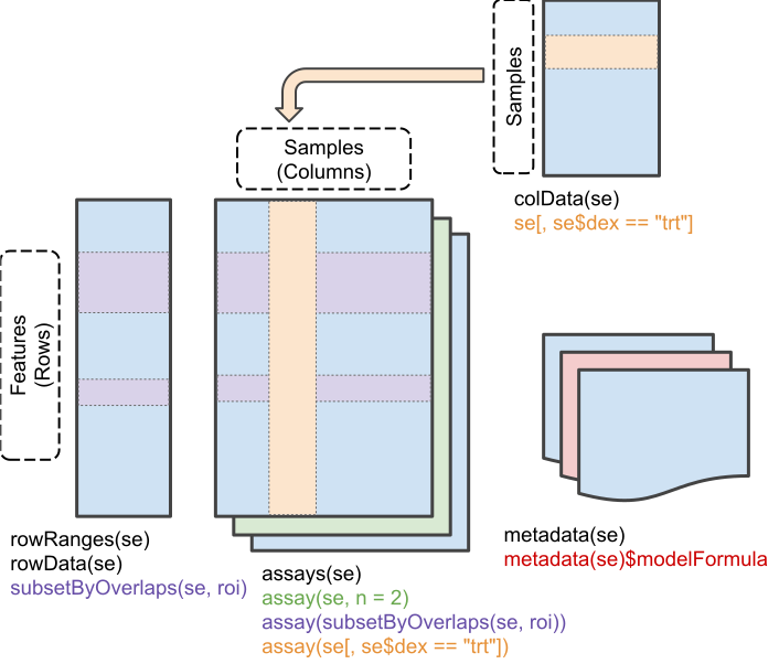
One of the most used Bioconductor S4 objects is the SummarizedExperiment, which was developed to hold any kind of data from features (e.g., genes, proteins, metabolites) measured across many samples, and also metadata about the features and samples. The following diagram shows how the different data slots in the SummarizedExperiment relate to each other.

We’ll take a look at data in a SummarizedExperiment object:

library(SummarizedExperiment)

SE <- readRDS(system.file("extdata/GSE96870_se.rds", package="bioc2026Intro"))
SE

## class: RangedSummarizedExperiment 
## dim: 41786 22 
## metadata(0):
## assays(1): counts
## rownames(41786): Xkr4 LOC105243853 ... TrnT TrnP
## rowData names(3): ENTREZID product gbkey
## colnames(22): GSM2545337 GSM2545338 ... GSM2545346 GSM2545347
## colData names(12): title geo_accession ... Label Group

Validation

The other big part of S4 objects is validation. This can be a bit hard to wrap your head around.

The Bioconductor designers put special validation checks on the input data for the Bioconductor objects when you load data into them.

The following is what is called the Constructor for the SummarizedExperiment object. This is what we use to make a brand new SummarizedExperiment object from its pieces.

SummarizedExperiment(assays=SimpleList(),
                     rowData=NULL, rowRanges=NULL,
                     colData=DataFrame(),
                     metadata=list(),
                     checkDimnames=TRUE)

Each argument to the SummarizedExperiment constructor defines restrictions on that slot. For example, there is a slot called assays.

The checkDimnames argument is critical. In order to do any work with an experiment you need to map samples to colNames (the experimental matrix). For example, to calculate differential expression between samples, you need to specify the different groups to compare and which samples map to which groups. Thus, the column names in the AssayData must be identical to the row names in colData.

If it isn’t in colData, it doesn’t exist

Keep in mind that your colData must be as complete as possible. Why? The short answer is that if there isn’t a row for your sample in colData, then it basically doesn’t exist for Bioconductor methods.

So make sure your colData contains sample names for all your samples.

In some ways, the SummarizedExperiment object is like a data.frame, but with extra metadata. For example, our object has column names, which correspond to sample identifiers:

colnames(SE)

##  [1] "GSM2545337" "GSM2545338" "GSM2545348" "GSM2545353" "GSM2545343"
##  [6] "GSM2545349" "GSM2545354" "GSM2545339" "GSM2545344" "GSM2545352"
## [11] "GSM2545362" "GSM2545340" "GSM2545345" "GSM2545350" "GSM2545363"
## [16] "GSM2545336" "GSM2545342" "GSM2545351" "GSM2545380" "GSM2545341"
## [21] "GSM2545346" "GSM2545347"

And row names:

rownames(SE)[1:30]

##  [1] "Xkr4"          "LOC105243853"  "LOC105242387"  "LOC105242467" 
##  [5] "Rp1"           "Sox17"         "Gm7357"        "LOC105243855" 
##  [9] "LOC105243854"  "Gm7369"        "Gm29874"       "Gm6123"       
## [13] "Mrpl15"        "Lypla1"        "LOC105243856"  "Tcea1"        
## [17] "Gm6104"        "Rgs20"         "Gm16041"       "Atp6v1h"      
## [21] "Oprk1"         "Npbwr1"        "4732440D04Rik" "Rb1cc1"       
## [25] "Fam150a"       "Gm2147"        "LOC102631893"  "St18"         
## [29] "LOC102641523"  "Pcmtd1"

So far, so good.

Assay Data

Everything in SummarizedExperiment is built around the Assay data that we store in it.

Each element of the Assay data list contains a matrix with the following contents:

• Rows: correspond to Gene Locus or possibly Transcripts
• Columns: correspond to the samples used in your experiment.
• Values: correspond to the actual data. In the case of RNAseq, these are the counts that map to each row.

You can extract the assay data using the assay() method:

assay_data <- assay(SE)
head(assay_data)

##              GSM2545337 GSM2545338 GSM2545348 GSM2545353 GSM2545343 GSM2545349
## Xkr4               2410       2159       2275       1910       2235       1881
## LOC105243853          0          1          1          0          3          0
## LOC105242387        121        110        161        214        130        154
## LOC105242467          5          5          2          1          2          4
## Rp1                   2          0          3          1          1          6
## Sox17               239        218        302        322        296        286
##              GSM2545354 GSM2545339 GSM2545344 GSM2545352 GSM2545362 GSM2545340
## Xkr4               1771       1980       1779       1890       2315       1977
## LOC105243853          0          4          3          1          1          0
## LOC105242387        124        120        131        272        189        172
## LOC105242467          4          5          2          3          2          2
## Rp1                   3          3          1          5          3          2
## Sox17               273        220        233        267        197        261
##              GSM2545345 GSM2545350 GSM2545363 GSM2545336 GSM2545342 GSM2545351
## Xkr4               1528       2584       1645       1891       1757       1837
## LOC105243853          0          0          0          0          1          1
## LOC105242387        160        124        223        204        177        221
## LOC105242467          2          7          1         12          3          1
## Rp1                   2          5          1          2          3          3
## Sox17               271        325        310        251        179        201
##              GSM2545380 GSM2545341 GSM2545346 GSM2545347
## Xkr4               1723       1945       1644       1585
## LOC105243853          1          0          1          3
## LOC105242387        251        173        180        176
## LOC105242467          4          6          1          2
## Rp1                   0          1          2          2
## Sox17               246        232        205        230

Assays Are Not just for RNAseq data

Assay Data is very flexible. For example, there are flow cytometry objects where the rows correspond to cell surface markers, and columns that correspond to each cell. Similarly, SingleCellExperiment objects (which are derived from SummarizedExperiment) have rows that correspond to Genes and columns that correspond to individual cells.

Think about it

Are the colnames of our object identical to the colnames of the assay object? Try it out:

colnames(SE)

##  [1] "GSM2545337" "GSM2545338" "GSM2545348" "GSM2545353" "GSM2545343"
##  [6] "GSM2545349" "GSM2545354" "GSM2545339" "GSM2545344" "GSM2545352"
## [11] "GSM2545362" "GSM2545340" "GSM2545345" "GSM2545350" "GSM2545363"
## [16] "GSM2545336" "GSM2545342" "GSM2545351" "GSM2545380" "GSM2545341"
## [21] "GSM2545346" "GSM2545347"

colnames(assay(SE))

##  [1] "GSM2545337" "GSM2545338" "GSM2545348" "GSM2545353" "GSM2545343"
##  [6] "GSM2545349" "GSM2545354" "GSM2545339" "GSM2545344" "GSM2545352"
## [11] "GSM2545362" "GSM2545340" "GSM2545345" "GSM2545350" "GSM2545363"
## [16] "GSM2545336" "GSM2545342" "GSM2545351" "GSM2545380" "GSM2545341"
## [21] "GSM2545346" "GSM2545347"

Metadata

Metadata is information about the experiment that is not part of the Assay Data.

The most important part of the metadata is the colData slot. This slot contains information about the samples (the columns) of the assay. This is where we store the Experimental Design that we talked about.

colData(SE)

## DataFrame with 22 rows and 12 columns
##                      title geo_accession     organism         age         sex
##                <character>   <character>  <character> <character> <character>
## GSM2545337 CNS_RNA-seq_11C    GSM2545337 Mus musculus     8 weeks      Female
## GSM2545338 CNS_RNA-seq_12C    GSM2545338 Mus musculus     8 weeks      Female
## GSM2545348 CNS_RNA-seq_27C    GSM2545348 Mus musculus     8 weeks      Female
## GSM2545353  CNS_RNA-seq_3C    GSM2545353 Mus musculus     8 weeks      Female
## GSM2545343 CNS_RNA-seq_20C    GSM2545343 Mus musculus     8 weeks        Male
## ...                    ...           ...          ...         ...         ...
## GSM2545351  CNS_RNA-seq_2C    GSM2545351 Mus musculus     8 weeks      Female
## GSM2545380  CNS_RNA-seq_9C    GSM2545380 Mus musculus     8 weeks      Female
## GSM2545341 CNS_RNA-seq_17C    GSM2545341 Mus musculus     8 weeks        Male
## GSM2545346 CNS_RNA-seq_25C    GSM2545346 Mus musculus     8 weeks        Male
## GSM2545347 CNS_RNA-seq_26C    GSM2545347 Mus musculus     8 weeks        Male
##              infection      strain        time      tissue     mouse
##            <character> <character> <character> <character> <integer>
## GSM2545337 NonInfected     C57BL/6        Day0  Cerebellum         9
## GSM2545338 NonInfected     C57BL/6        Day0  Cerebellum        10
## GSM2545348 NonInfected     C57BL/6        Day0  Cerebellum         8
## GSM2545353 NonInfected     C57BL/6        Day0  Cerebellum         4
## GSM2545343 NonInfected     C57BL/6        Day0  Cerebellum        11
## ...                ...         ...         ...         ...       ...
## GSM2545351  InfluenzaA     C57BL/6        Day8  Cerebellum        16
## GSM2545380  InfluenzaA     C57BL/6        Day8  Cerebellum        19
## GSM2545341  InfluenzaA     C57BL/6        Day8  Cerebellum         6
## GSM2545346  InfluenzaA     C57BL/6        Day8  Cerebellum        23
## GSM2545347  InfluenzaA     C57BL/6        Day8  Cerebellum        24
##                     Label       Group
##                  <factor>    <factor>
## GSM2545337 Female_Day0_9  Female_Day0
## GSM2545338 Female_Day0_10 Female_Day0
## GSM2545348 Female_Day0_8  Female_Day0
## GSM2545353 Female_Day0_4  Female_Day0
## GSM2545343 Male_Day0_11   Male_Day0  
## ...                   ...         ...
## GSM2545351 Female_Day8_16 Female_Day8
## GSM2545380 Female_Day8_19 Female_Day8
## GSM2545341 Male_Day8_6    Male_Day8  
## GSM2545346 Male_Day8_23   Male_Day8  
## GSM2545347 Male_Day8_24   Male_Day8

In our experimental design, we have males and females, timepoints, and different kinds of tissues.

Think about it

What do the rownames() of colData(SE) correspond to?

rownames(colData(SE))

##  [1] "GSM2545337" "GSM2545338" "GSM2545348" "GSM2545353" "GSM2545343"
##  [6] "GSM2545349" "GSM2545354" "GSM2545339" "GSM2545344" "GSM2545352"
## [11] "GSM2545362" "GSM2545340" "GSM2545345" "GSM2545350" "GSM2545363"
## [16] "GSM2545336" "GSM2545342" "GSM2545351" "GSM2545380" "GSM2545341"
## [21] "GSM2545346" "GSM2545347"

Keep your SummarizedExperiment whole

It might be tempting to extract the assay data and the metadata and work with them separately. But as we’ll see in the following section, these two slots work together and enable all sorts of analysis.

Subsetting SummarizedExperiment

We saw that we have the checkNames constraint. This is because we can use the colData and the assayData in our object to do subsetting using the metadata.

female <- SE[,SE$sex == "Female"]
female

## class: RangedSummarizedExperiment 
## dim: 41786 12 
## metadata(0):
## assays(1): counts
## rownames(41786): Xkr4 LOC105243853 ... TrnT TrnP
## rowData names(3): ENTREZID product gbkey
## colnames(12): GSM2545337 GSM2545338 ... GSM2545351 GSM2545380
## colData names(12): title geo_accession ... Label Group

colData(female)

## DataFrame with 12 rows and 12 columns
##                      title geo_accession     organism         age         sex
##                <character>   <character>  <character> <character> <character>
## GSM2545337 CNS_RNA-seq_11C    GSM2545337 Mus musculus     8 weeks      Female
## GSM2545338 CNS_RNA-seq_12C    GSM2545338 Mus musculus     8 weeks      Female
## GSM2545348 CNS_RNA-seq_27C    GSM2545348 Mus musculus     8 weeks      Female
## GSM2545353  CNS_RNA-seq_3C    GSM2545353 Mus musculus     8 weeks      Female
## GSM2545339 CNS_RNA-seq_13C    GSM2545339 Mus musculus     8 weeks      Female
## ...                    ...           ...          ...         ...         ...
## GSM2545362  CNS_RNA-seq_5C    GSM2545362 Mus musculus     8 weeks      Female
## GSM2545336 CNS_RNA-seq_10C    GSM2545336 Mus musculus     8 weeks      Female
## GSM2545342  CNS_RNA-seq_1C    GSM2545342 Mus musculus     8 weeks      Female
## GSM2545351  CNS_RNA-seq_2C    GSM2545351 Mus musculus     8 weeks      Female
## GSM2545380  CNS_RNA-seq_9C    GSM2545380 Mus musculus     8 weeks      Female
##              infection      strain        time      tissue     mouse
##            <character> <character> <character> <character> <integer>
## GSM2545337 NonInfected     C57BL/6        Day0  Cerebellum         9
## GSM2545338 NonInfected     C57BL/6        Day0  Cerebellum        10
## GSM2545348 NonInfected     C57BL/6        Day0  Cerebellum         8
## GSM2545353 NonInfected     C57BL/6        Day0  Cerebellum         4
## GSM2545339  InfluenzaA     C57BL/6        Day4  Cerebellum        15
## ...                ...         ...         ...         ...       ...
## GSM2545362  InfluenzaA     C57BL/6        Day4  Cerebellum        20
## GSM2545336  InfluenzaA     C57BL/6        Day8  Cerebellum        14
## GSM2545342  InfluenzaA     C57BL/6        Day8  Cerebellum         5
## GSM2545351  InfluenzaA     C57BL/6        Day8  Cerebellum        16
## GSM2545380  InfluenzaA     C57BL/6        Day8  Cerebellum        19
##                     Label       Group
##                  <factor>    <factor>
## GSM2545337 Female_Day0_9  Female_Day0
## GSM2545338 Female_Day0_10 Female_Day0
## GSM2545348 Female_Day0_8  Female_Day0
## GSM2545353 Female_Day0_4  Female_Day0
## GSM2545339 Female_Day4_15 Female_Day4
## ...                   ...         ...
## GSM2545362 Female_Day4_20 Female_Day4
## GSM2545336 Female_Day8_14 Female_Day8
## GSM2545342 Female_Day8_5  Female_Day8
## GSM2545351 Female_Day8_16 Female_Day8
## GSM2545380 Female_Day8_19 Female_Day8

This tight interaction of metadata and assay data is critical when we start doing differential analysis. The experimental design will help determine whether we can make the comparisons we want to make and the conclusions we can draw from the dataset.

Remember the Comma

Remember that the , (comma) is used to distinguish between rows and columns. Rows correspond to genes and columns correpsond to samples.

In the above example, we are subsetting the samples, so our criteria goes after the comma.

This is the base R way of subsetting the SummarizedExperiment object. In a later section, we will learn how to use the tidySummarizedExperiment package to subset/manipulate/plot it the tidyverse way - essentially this package lets us use dplyr on the SummarizedExperiment and DESeqDataset objects.

Try it out

Try subsetting SE to have time == "Day0". How many samples are left?

day0 <- SE[,SE$----- == -------]
day0
colData(day0)

rowData: Additional Annotations

rowData(SE)

## DataFrame with 41786 rows and 3 columns
##                 ENTREZID                product       gbkey
##              <character>            <character> <character>
## Xkr4              497097 X Kell blood group p..        mRNA
## LOC105243853   105243853 uncharacterized LOC1..       ncRNA
## LOC105242387   105242387 uncharacterized LOC1..       ncRNA
## LOC105242467   105242467 lipoxygenase homolog..        mRNA
## Rp1                19888 retinitis pigmentosa..        mRNA
## ...                  ...                    ...         ...
## TrnS2              17743               tRNA-Ser        tRNA
## TrnL2              17736               tRNA-Leu        tRNA
## TrnE               17729               tRNA-Glu        tRNA
## TrnT               17744               tRNA-Thr        tRNA
## TrnP               17739               tRNA-Pro        tRNA

rowRanges: Genomic Information

The SummarizedExperiment we are working with is actually a variant: a RangedSummarizedExperiment. It contains an additional slot called rowRanges. The rowRanges slot of a SummarizedExperiment can contain genomic information, such as genomic coordinates. Let’s take a look:

rowRanges(SE)

## GRanges object with 41786 ranges and 3 metadata columns:
##                seqnames          ranges strand |    ENTREZID
##                   <Rle>       <IRanges>  <Rle> | <character>
##           Xkr4        1 3670552-3671742      - |      497097
##   LOC105243853        1 3357323-3366505      + |   105243853
##   LOC105242387        1 3658847-3670456      - |   105242387
##   LOC105242467        1 4233436-4233728      - |   105242467
##            Rp1        1 4409170-4409241      - |       19888
##            ...      ...             ...    ... .         ...
##          TrnS2       MT     11613-11671      + |       17743
##          TrnL2       MT     11671-11741      + |       17736
##           TrnE       MT     14071-14139      - |       17729
##           TrnT       MT     15289-15355      + |       17744
##           TrnP       MT     15356-15422      - |       17739
##                               product       gbkey
##                           <character> <character>
##           Xkr4 X Kell blood group p..        mRNA
##   LOC105243853 uncharacterized LOC1..       ncRNA
##   LOC105242387 uncharacterized LOC1..       ncRNA
##   LOC105242467 lipoxygenase homolog..        mRNA
##            Rp1 retinitis pigmentosa..        mRNA
##            ...                    ...         ...
##          TrnS2               tRNA-Ser        tRNA
##          TrnL2               tRNA-Leu        tRNA
##           TrnE               tRNA-Glu        tRNA
##           TrnT               tRNA-Thr        tRNA
##           TrnP               tRNA-Pro        tRNA
##   -------
##   seqinfo: 90 sequences from an unspecified genome; no seqlengths

The seqnames column corresponds to the chromosome, ranges is what is called an IRanges object, which specifies an interval defined by a start and end coordinate, and a strand.

Filtering by Genomic Ranges

The SummarizedExperiment we are working with is actually a variant: a RangedSummarizedExperiment. This allows you to subset the rows by genomic intervals.

Our main technique for subsetting by i is subsetByOverlaps(). We’ll need to define a Genomic Region of Interest (ROI), and then we can subset our SE object with that ROI.

Our ROI is defined by a GRanges object, which can specify a range of genomic coordinates. Remember that the seqnames column corresponds to chromosome, and the ranges column needs to be defined as an IRanges() object, with a start and end.

roi <- GRanges(seqnames = "1", ranges=IRanges(start = 1, end = 5000000))
subset_SE <- subsetByOverlaps(SE, roi) 
subset_SE

## class: RangedSummarizedExperiment 
## dim: 19 22 
## metadata(0):
## assays(1): counts
## rownames(19): Xkr4 LOC105243853 ... Rgs20 Gm16041
## rowData names(3): ENTREZID product gbkey
## colnames(22): GSM2545337 GSM2545338 ... GSM2545346 GSM2545347
## colData names(12): title geo_accession ... Label Group

You can see we have 19 rows left in subset_SE that map to our Genomic Range of interest.

If you have more than 1 region of interest, you can combine multiple sets of ranges into your GRanges object for subsetting.

A Common Bioconductor Pattern

Depending on the package, we will tend to overwrite objects as we run methods on them, such as the following.

In DESeq2, each method will add something to the object (usually extra columns or a results table).

Here’s an example:

library(SummarizedExperiment)
library(DESeq2)

DSE <- DESeqDataSet(SE, design = ~ sex + time)  #make DESeqDataset
DSE <- DSE[rowSums(assay(DSE)) > 5,] #filter out low expressing candidates
DSE <- DESeq(DSE) #run estimateSizeFactors, estimateDispersions, nbinomialWaldTest

tidySummarizedExperiment

The SummarizedExperiment object does not act like the normal data.frame/tibble we expect, especially in filtering and subsetting.

The tidySummarizedExperiment package will be helpful for us to understand and visualize the SummarizedExperiment package. Once we do that, our SummarizedExperiment object will act more like a data.frame.

Basically, tidySummarizedExperiment treats the data as a long data frame that combines both the assay and metadata. This format is helpful in doing more work with the tidyverse:

library(tidySummarizedExperiment)

## Loading required package: ttservice

## tidySummarizedExperiment says: Printing is now handled externally. If you want to visualize the data in a tidy way, do library(tidyprint). See https://github.com/tidyomics/tidyprint for more information.

## 
## Attaching package: 'tidySummarizedExperiment'

## The following object is masked from 'package:generics':
## 
##     tidy

library(tidyprint)

## Registered S3 method overwritten by 'tidyprint':
##   method                         from                    
##   as_tibble.SummarizedExperiment tidySummarizedExperiment

tidy_print_on()

## ℹ tidyprint says: Tidy print enabled for this session only. Use tidy_print_on(remember = TRUE) to save this setting for future sessions.

SE

## # A SummarizedExperiment-tibble abstraction: Features=41786 | Samples=22 | 
## #   Assays=counts
## #                                     |--------------- COVARIATES -------------|
##        .feature     .sample  | counts | title geo_accession organism age   sex  
##        <chr>        <chr>    | <chr>  | <chr> <chr>         <chr>    <chr> <chr>
## 1      Xkr4         GSM2545… | 2410   | CNS_… GSM2545337    Mus mus… 8 we… Fema…
## 2      LOC105243853 GSM2545… | 0      | CNS_… GSM2545337    Mus mus… 8 we… Fema…
## 3      LOC105242387 GSM2545… | 121    | CNS_… GSM2545337    Mus mus… 8 we… Fema…
## 4      LOC105242467 GSM2545… | 5      | CNS_… GSM2545337    Mus mus… 8 we… Fema…
## 5      Rp1          GSM2545… | 2      | CNS_… GSM2545337    Mus mus… 8 we… Fema…
##        --------     -------  - ------ - ----- ------------- -------- ---   ---  
## 919288 TrnS2        GSM2545… | 2      | CNS_… GSM2545347    Mus mus… 8 we… Male 
## 919289 TrnL2        GSM2545… | 188    | CNS_… GSM2545347    Mus mus… 8 we… Male 
## 919290 TrnE         GSM2545… | 312    | CNS_… GSM2545347    Mus mus… 8 we… Male 
## 919291 TrnT         GSM2545… | 382    | CNS_… GSM2545347    Mus mus… 8 we… Male 
## 919292 TrnP         GSM2545… | 228    | CNS_… GSM2545347    Mus mus… 8 we… Male 
## # ℹ 11 more variables: infection <chr>, strain <chr>, time <chr>, tissue <chr>,
## #   mouse <chr>, Label <fct>, Group <fct>, `|` <|>, ENTREZID <chr>,
## #   product <chr>, gbkey <chr>

Filtering Data

We can use dplyr to filter the data using the tidySummarizedExperiment package:

SE |>
  filter(sex == "Female")

## # A SummarizedExperiment-tibble abstraction: Features=41786 | Samples=12 | 
## #   Assays=counts
## #                                     |--------------- COVARIATES -------------|
##        .feature     .sample  | counts | title geo_accession organism age   sex  
##        <chr>        <chr>    | <chr>  | <chr> <chr>         <chr>    <chr> <chr>
## 1      Xkr4         GSM2545… | 2410   | CNS_… GSM2545337    Mus mus… 8 we… Fema…
## 2      LOC105243853 GSM2545… | 0      | CNS_… GSM2545337    Mus mus… 8 we… Fema…
## 3      LOC105242387 GSM2545… | 121    | CNS_… GSM2545337    Mus mus… 8 we… Fema…
## 4      LOC105242467 GSM2545… | 5      | CNS_… GSM2545337    Mus mus… 8 we… Fema…
## 5      Rp1          GSM2545… | 2      | CNS_… GSM2545337    Mus mus… 8 we… Fema…
##        --------     -------  - ------ - ----- ------------- -------- ---   ---  
## 501428 TrnS2        GSM2545… | 3      | CNS_… GSM2545380    Mus mus… 8 we… Fema…
## 501429 TrnL2        GSM2545… | 215    | CNS_… GSM2545380    Mus mus… 8 we… Fema…
## 501430 TrnE         GSM2545… | 524    | CNS_… GSM2545380    Mus mus… 8 we… Fema…
## 501431 TrnT         GSM2545… | 551    | CNS_… GSM2545380    Mus mus… 8 we… Fema…
## 501432 TrnP         GSM2545… | 424    | CNS_… GSM2545380    Mus mus… 8 we… Fema…
## # ℹ 11 more variables: infection <chr>, strain <chr>, time <chr>, tissue <chr>,
## #   mouse <chr>, Label <fct>, Group <fct>, `|` <|>, ENTREZID <chr>,
## #   product <chr>, gbkey <chr>

Getting Counts across the experiment

We can produce summaries of the counts of each sample library:

SE |>
    group_by(.sample) |>
    summarise(total_counts=sum(counts))

## tidySummarizedExperiment says: A data frame is returned for independent data analysis.

## Warning: `when()` was deprecated in purrr 1.0.0.
## ℹ Please use `if` instead.
## ℹ The deprecated feature was likely used in the tidySummarizedExperiment
##   package.
##   Please report the issue at
##   <https://github.com/stemangiola/tidySummarizedExperiment/issues>.
## This warning is displayed once per session.
## Call `lifecycle::last_lifecycle_warnings()` to see where this warning was
## generated.

## # A tibble: 22 × 2
##    .sample    total_counts
##    <chr>             <int>
##  1 GSM2545336     40265225
##  2 GSM2545337     33818586
##  3 GSM2545338     31684299
##  4 GSM2545339     32663438
##  5 GSM2545340     33518799
##  6 GSM2545341     32777049
##  7 GSM2545342     31624027
##  8 GSM2545343     40031023
##  9 GSM2545344     33726110
## 10 GSM2545345     34043596
## # ℹ 12 more rows

Try it out

Try summarizing the total_counts by sex or by infection:

SE |>
  group_by(sex) |>
  summarize(total_counts = sum(counts))

## tidySummarizedExperiment says: A data frame is returned for independent data analysis.

## # A tibble: 2 × 2
##   sex    total_counts
##   <chr>         <int>
## 1 Female    440881903
## 2 Male      362166871

Plotting

We can look at the distribution of counts across samples by using .sample as our grouping variable in ggplot().

SE |>
    ggplot(aes(counts + 1, group=.sample, color=infection)) +
    geom_density() +
    scale_x_log10() +
    theme_bw()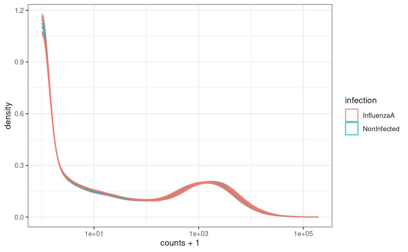

Our data (individual gene counts) is highly skewed. If we log-transform the data, then the skew is lessened. The boxplots of log counts are helpful for detecting batch effects.

SE |>
    ggplot(aes(y=log2(counts + 1), group=.sample, fill=infection)) +
    geom_boxplot() +
    theme_bw()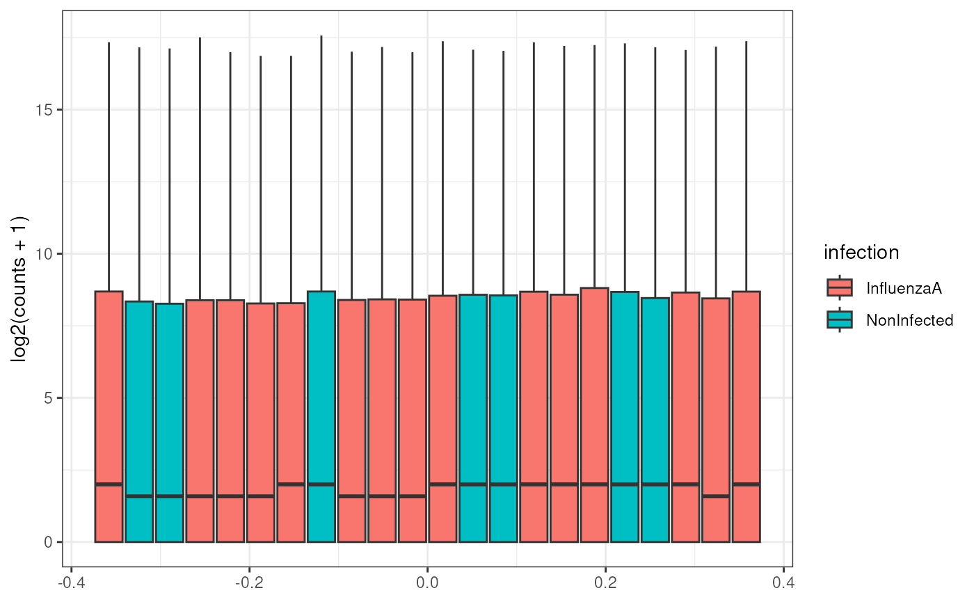

Take a look at the above box plot. Are there differences in distribution between samples?

In order to compare expression levels between samples, we will need to adjust, or normalize by library size. We’ll investigate this further when we get to differential expression.

Try it Out

Try mapping another variable to fill.

SE |>
    ggplot(aes(y=log2(counts + 1), group=.sample, fill=sex)) +
    geom_boxplot() +
    theme_bw()

Take Home Messages

• We package multiple parts of the data (assay data and metadata) into a SummarizedExperiment object:
  • Columns correspond to samples, Rows correspond to gene locus or transcripts
  • Column names of the assay data must match a column in the colData
  • Experimental Design variables are part of the colData
  • Rownames of the assay data must match the rowNames in the column data
• The SummarizedExperiment object lets us subset by phenotype variables
• tidySummarizedExperiment lets us interact with the SummarizedExperiment object as if it were a long data frame with both metadata and assay data together.
  • We can plot and subset the SummarizedExperiment object using our regular tidyverse tools (ggplot2, dplyr, etc.) once we load the tidySummarizedExperiment package.

What about all of the other kinds of objects?

Most of the other Bioconductor Data Structures derive from some variant of the SummarizedExperiment, or are utilized by SummarizedExperiment, such as GenomicRanges. They might add some functionality that is core to the package they belong to, such as DEseq2. This includes seurat objects for Single Cell sequencing.

Please see the Installing vignette for more information.

---

1. The Bioconductor project was initiated by Robert Gentleman, one of the two creators of the R language. Bioconductor provides tools dedicated to omics data analysis. Bioconductor uses the R statistical programming language and is open source and open development.↩︎