A Full Workflow in Bioconductor
In this document, we run a full analysis on our
RangedSummarizedExperiment by prerprocessing and running
DESeq() on the data. We then plot our candidates using the
EnhancedVolcano package.
## Loading required package: MatrixGenerics## Loading required package: matrixStats##
## Attaching package: 'MatrixGenerics'## The following objects are masked from 'package:matrixStats':
##
## colAlls, colAnyNAs, colAnys, colAvgsPerRowSet, colCollapse,
## colCounts, colCummaxs, colCummins, colCumprods, colCumsums,
## colDiffs, colIQRDiffs, colIQRs, colLogSumExps, colMadDiffs,
## colMads, colMaxs, colMeans2, colMedians, colMins, colOrderStats,
## colProds, colQuantiles, colRanges, colRanks, colSdDiffs, colSds,
## colSums2, colTabulates, colVarDiffs, colVars, colWeightedMads,
## colWeightedMeans, colWeightedMedians, colWeightedSds,
## colWeightedVars, rowAlls, rowAnyNAs, rowAnys, rowAvgsPerColSet,
## rowCollapse, rowCounts, rowCummaxs, rowCummins, rowCumprods,
## rowCumsums, rowDiffs, rowIQRDiffs, rowIQRs, rowLogSumExps,
## rowMadDiffs, rowMads, rowMaxs, rowMeans2, rowMedians, rowMins,
## rowOrderStats, rowProds, rowQuantiles, rowRanges, rowRanks,
## rowSdDiffs, rowSds, rowSums2, rowTabulates, rowVarDiffs, rowVars,
## rowWeightedMads, rowWeightedMeans, rowWeightedMedians,
## rowWeightedSds, rowWeightedVars## Loading required package: GenomicRanges## Loading required package: stats4## Loading required package: BiocGenerics## Loading required package: generics##
## Attaching package: 'generics'## The following objects are masked from 'package:base':
##
## as.difftime, as.factor, as.ordered, intersect, is.element, setdiff,
## setequal, union##
## Attaching package: 'BiocGenerics'## The following objects are masked from 'package:stats':
##
## IQR, mad, sd, var, xtabs## The following object is masked from 'package:utils':
##
## data## The following objects are masked from 'package:base':
##
## anyDuplicated, aperm, append, as.data.frame, basename, cbind,
## colnames, dirname, do.call, duplicated, eval, evalq, Filter, Find,
## get, grep, grepl, is.unsorted, lapply, Map, mapply, match, mget,
## order, paste, pmax, pmax.int, pmin, pmin.int, Position, rank,
## rbind, Reduce, rownames, sapply, saveRDS, scale, sequence, table,
## tapply, transform, unique, unsplit, which.max, which.min## Loading required package: S4Vectors##
## Attaching package: 'S4Vectors'## The following object is masked from 'package:utils':
##
## findMatches## The following objects are masked from 'package:base':
##
## expand.grid, I, unname## Loading required package: IRanges## Loading required package: Seqinfo## Loading required package: Biobase## Welcome to Bioconductor
##
## Vignettes contain introductory material; view with
## 'browseVignettes()'. To cite Bioconductor, see
## 'citation("Biobase")', and for packages 'citation("pkgname")'.##
## Attaching package: 'Biobase'## The following object is masked from 'package:MatrixGenerics':
##
## rowMedians## The following objects are masked from 'package:matrixStats':
##
## anyMissing, rowMedians## Loading required package: ttservice## tidySummarizedExperiment says: Printing is now handled externally. If you want to visualize the data in a tidy way, do library(tidyprint). See https://github.com/tidyomics/tidyprint for more information.##
## Attaching package: 'tidySummarizedExperiment'## The following object is masked from 'package:generics':
##
## tidy## ── Attaching core tidyverse packages ──────────────────────── tidyverse 2.0.0 ──
## ✔ forcats 1.0.1 ✔ readr 2.2.0
## ✔ lubridate 1.9.5 ✔ stringr 1.6.0
## ✔ purrr 1.2.2 ✔ tibble 3.3.1## ── Conflicts ────────────────────────────────────────── tidyverse_conflicts() ──
## ✖ lubridate::%within%() masks IRanges::%within%()
## ✖ dplyr::bind_cols() masks ttservice::bind_cols()
## ✖ dplyr::bind_rows() masks ttservice::bind_rows()
## ✖ dplyr::collapse() masks IRanges::collapse()
## ✖ dplyr::combine() masks Biobase::combine(), BiocGenerics::combine()
## ✖ dplyr::count() masks matrixStats::count()
## ✖ dplyr::desc() masks IRanges::desc()
## ✖ tidyr::expand() masks S4Vectors::expand()
## ✖ dplyr::filter() masks stats::filter()
## ✖ dplyr::first() masks S4Vectors::first()
## ✖ dplyr::lag() masks stats::lag()
## ✖ ggplot2::Position() masks BiocGenerics::Position(), base::Position()
## ✖ purrr::reduce() masks GenomicRanges::reduce(), IRanges::reduce()
## ✖ dplyr::rename() masks S4Vectors::rename()
## ✖ lubridate::second() masks S4Vectors::second()
## ✖ lubridate::second<-() masks S4Vectors::second<-()
## ✖ dplyr::slice() masks IRanges::slice()
## ℹ Use the conflicted package (<http://conflicted.r-lib.org/>) to force all conflicts to become errors## Loading required package: ggrepel
GSE96870 <- readRDS(system.file("extdata/GSE96870_se.rds", package="bioc2026Intro"))
GSE96870
## class: RangedSummarizedExperiment
## dim: 41786 22
## metadata(0):
## assays(1): counts
## rownames(41786): Xkr4 LOC105243853 ... TrnT TrnP
## rowData names(3): ENTREZID product gbkey
## colnames(22): GSM2545337 GSM2545338 ... GSM2545346 GSM2545347
## colData names(12): title geo_accession ... Label GroupPreprocessing and Filtering
We first need to convert our RangedSummarizedExperiment
object into a DESeq2 object, which we do by specifying the
design formula.
Then we can filter out genes by low total expression counts (5 counts or less).
GSE96870_deseq <-
  DESeqDataSet(GSE96870, design = ~ sex + time)  #make DESeqDataset
## Warning in DESeqDataSet(GSE96870, design = ~sex + time): some variables in
## design formula are characters, converting to factorsRun DESeq
The DESeq() function will preprocess our data by
estimating the size factors of each sample, allowing us to normalize
each sample by library size. The actual modeling of the expression
candidates is done by nbinomialWaldTest.
GSE96870_fit <- DESeq(GSE96870_filtered) #run estimateSizeFactors, estimateDispersions, nbinomialWaldTest## estimating size factors## estimating dispersions## gene-wise dispersion estimates## mean-dispersion relationship## final dispersion estimates## fitting model and testingFilter Results by Alpha, Visualize
We use the results() function in DESeq2 to
filter our candidates using an alpha threshold of 0.05 and a log-fold
change threshold of 1 (which corresponds to a 2 fold expression
difference between our two conditions, “Day0”, and “Day8”).
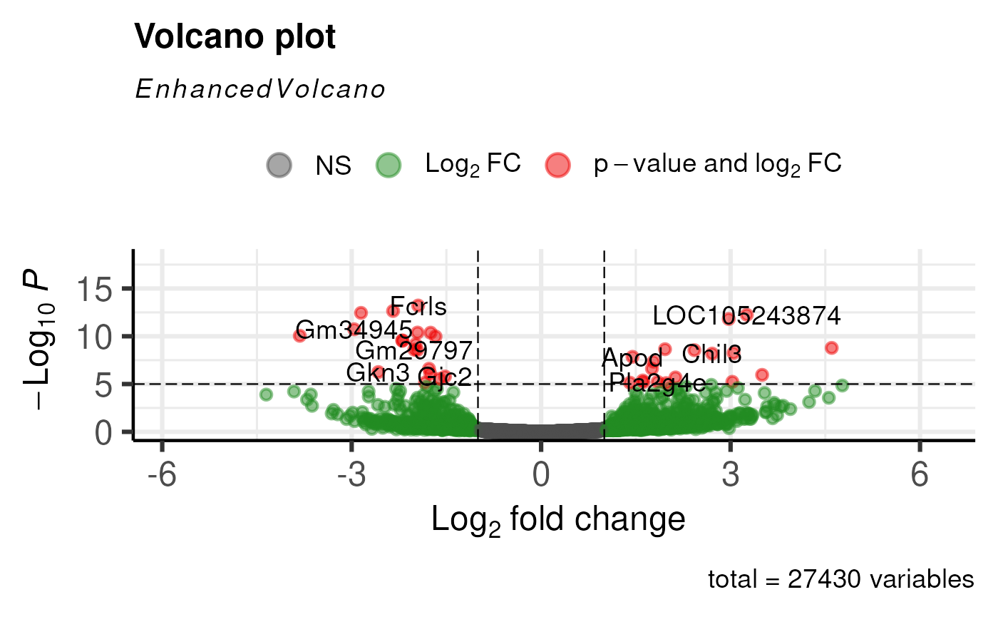
Finally, we can take those candidates and then plot a volcano plot to visualize -log2 fold-change versus -log10 p-value.
GSE_results <- results(GSE96870_fit,
                       contrast = c("time", "Day8", "Day0"),
                       lfcThreshold = 1,
                       alpha = 0.05) #calculate results from the contrast

GSE_results
## log2 fold change (MLE): time Day8 vs Day0
## Wald test p-value: time Day8 vs Day0
## DataFrame with 27430 rows and 6 columns
## baseMean log2FoldChange lfcSE stat pvalue padj
## <numeric> <numeric> <numeric> <numeric> <numeric> <numeric>
## Xkr4 1937.755565 -0.235730 0.108040 -2.181883 1.000000 1
## LOC105243853 0.962588 0.525506 1.189708 0.441710 0.754869 NA
## LOC105242387 169.913400 0.456042 0.138527 3.292070 0.999957 1
## LOC105242467 3.435073 0.273173 0.583568 0.468108 0.908089 1
## Rp1 2.273456 -0.259292 0.682140 -0.380116 0.893669 1
## ... ... ... ... ... ... ...
## TrnS2 1.76325 0.7843260 0.710962 1.103189 0.625231 1
## TrnL2 169.37651 0.4982649 0.100922 4.937145 1.000000 1
## TrnE 335.92910 0.1635685 0.199436 0.820154 0.999986 1
## TrnT 379.46721 0.4187775 0.109323 3.830656 1.000000 1
## TrnP 277.35435 0.0737642 0.224201 0.329010 0.999983 1
EnhancedVolcano(GSE_results,
                lab = rownames(GSE_results),
                x = 'log2FoldChange',
                y = 'pvalue')
## Warning: Using `size` aesthetic for lines was deprecated in ggplot2 3.4.0.
## ℹ Please use `linewidth` instead.
## ℹ The deprecated feature was likely used in the EnhancedVolcano package.
## Please report the issue to the authors.
## This warning is displayed once per session.
## Call `lifecycle::last_lifecycle_warnings()` to see where this warning was
## generated.## Warning: The `size` argument of `element_line()` is deprecated as of ggplot2 3.4.0.
## ℹ Please use the `linewidth` argument instead.
## ℹ The deprecated feature was likely used in the EnhancedVolcano package.
## Please report the issue to the authors.
## This warning is displayed once per session.
## Call `lifecycle::last_lifecycle_warnings()` to see where this warning was
## generated.