Chapter 5 R Markdown Reports

Learning objectives are to be able to: Explain why R Markdown files are useful for creating data analysis reports. Recognize how to test pieces of code within R Markdown files. Recognize how to create a full R Markdown file report in html and other formats. Explain that R Markdowns generate reports from code in a way that is a bit closer to someone else trying your code.

5.1 Reports support reproducibility

Using R Markdown files helps you to create supports that can more transparently show what you did for your analysis and it can help you to test that your code works as expected. Scripts allow you to save code, but they do not allow you to have the following additional benefits.

The following are reasons why R Markdown files help reproducibility:

They allow you to show and share your code and the output of your code in one place! (this can be done in several ways depending on what you want)
They allow you to test if your code works outside of what is active in your environment
They allow you to test sections and all previous sections of your code out to troubleshoot
They help you understand what might be wrong with your code in smaller sections of code if you have an issue

5.2 Getting Started with R Markdown

OK, so now we know how to make a new R Markdown file from the previous section.

Click here for a review on how to create R Markdown files in RStudio.

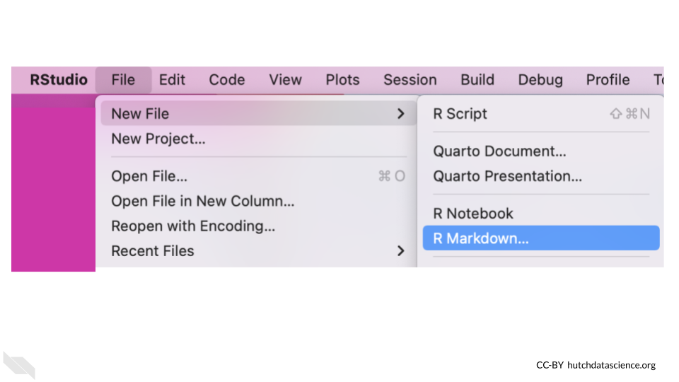
To open a new R Markdown file by go to File –> New File –>R Markdown in the upper menu of RStudio.

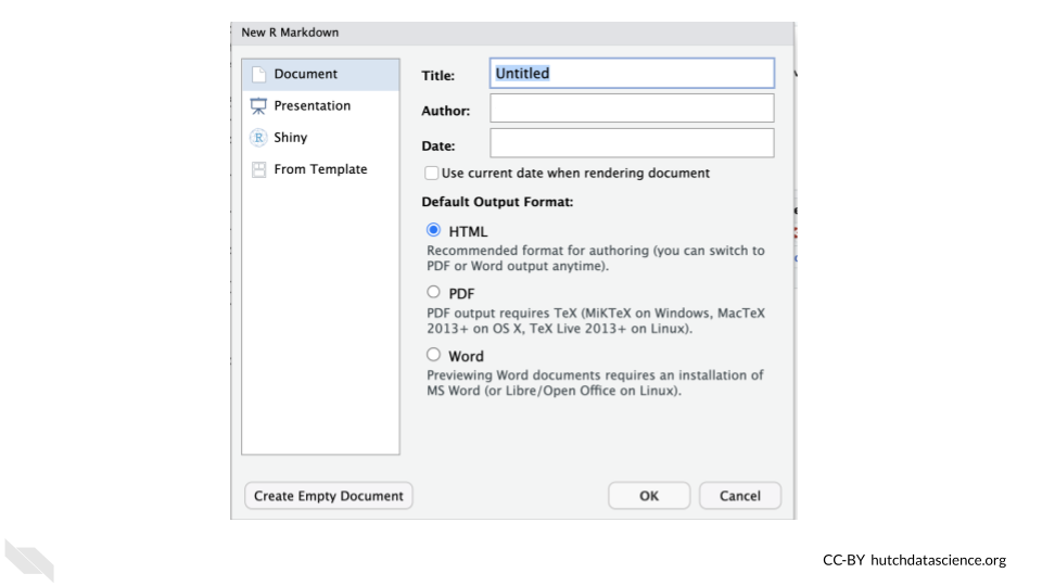
Creating an R Markdown file in R Studio by selecting File, New File, R Markdown.

Creating an R Markdown file starts with a pop-up and you can simply click the OK button.

The new pane will open on the upper left.

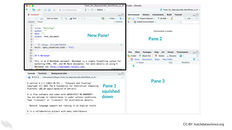
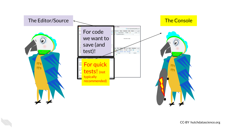
This pane is where we can write code to save in our R Markdown report.

Thus the lower left pane is where we can test out code (although we do not generally recommend it), but the top pane is where we can write code that we wish to save.

Note that you can also test selected code (or a current line) in an R Markdown file using a keyboard shortcut of Ctrl+Enter on Windows & Linux computers or Cmd+Return on Mac computers.

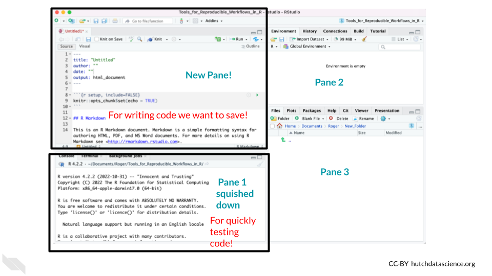
The new pane will open on the upper left and is for writing code we want to save, while the bottom pane is for writing code we want to test.

The top pane where we save code is called the editor. The lower pane where we test code is called the console.

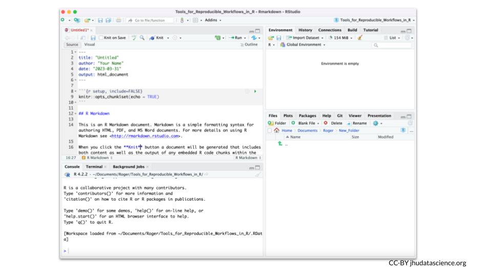
The editor in the top left, also called source, is where we write code we want to save. The lower left is the console where we do quick tests of our code.

Once open the file your RStudio should look something like this:

Example of how RStudio looks when you open a new R Markdown file.

5.3 Rendering R Markdown files

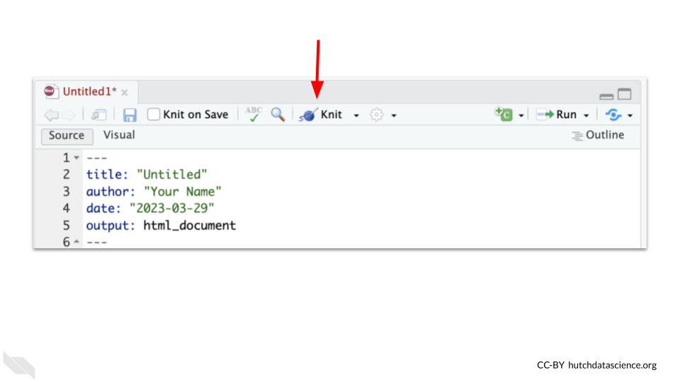
There is a special Knit button that looks like a ball of yarn with a knitting needle at the top of the R Markdown files that helps you create your report. Since R Markdown files by default have some code, we can press this to see what a rendered report might look like before we start writing our own code.

The Knit button at the top of the R Markdown file allows us to create a nice report from the file.

You will likely be prompted to give the file a name after you press the Knit button and to confirm where you want to save the rendered version.

You will then see in a second or two (after some information is printed on the Render tab in the lower left pane) a screen pop up with the rendered version of the report.

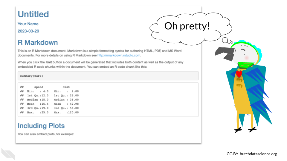
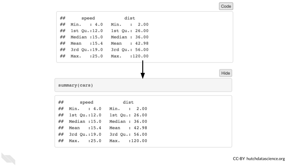
This will look something like this:

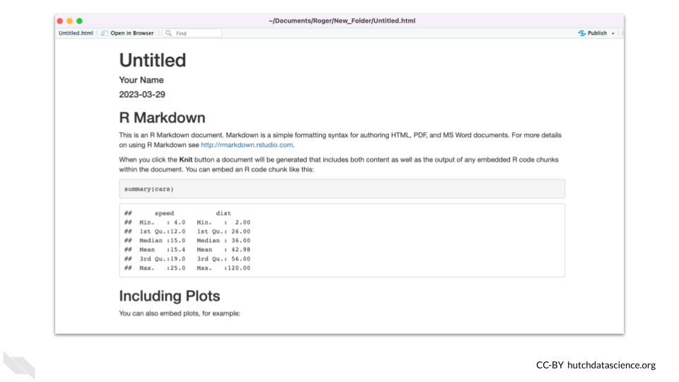
Rendered R Markdown example after pressing the Knit button after making a new R Markdown file.

Here we can see that there are some headers and text information, as well as some code shown in the gray box. We also see that this code is followed by the output of the code, where we see a summary of the cars dataset.

If you scroll down you will see an example of what a plot looks like in such a report.

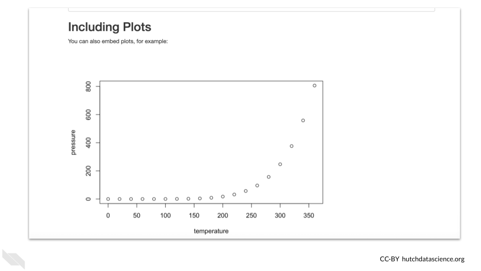
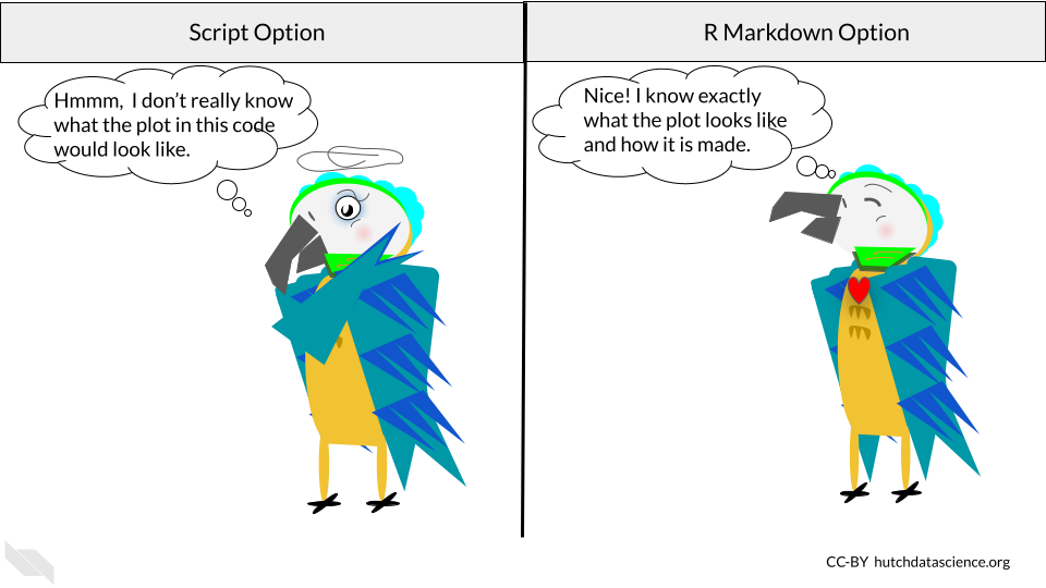
An image of the plot that is included in R Markdown files by default if you scroll down in the rendered report.

Hopefully you can already start to appreciate how useful it can be to send people a report of your code with the output of your code and plots, as opposed to just a simple script, which can’t show the output of our code!

A cartoon showing the parrot being confused about what a plot might look like from a script and happy about knowing how a plot looks and what code it took to create it with an R Markdown file

It’s important to note that when we knit an R Markdown file, it will test our code as if we have an empty environment and it will rely on only the code written in the R Markdown file. It can’t use code that was tested in the Console or run interactively in the R Markdown file (more on that soon).

This process really helps with reproducibility because it helps us make sure that all the instructions needed (loading packages, assigning objects, etc) are within the code that we saved in the R Markdown file.

If anything is missing, the file will either not knit and you will get an error, or you may see that the output of the code is different than you expected.

Now let’s discuss how to start writing code in such a file.

5.4 Writing code in R Markdown files

5.4.1 The YAML

At the top of an R Markdown file you will see some special code that is called YAML code. It is commonly used to configure programming projects. It does the same for our R Markdown reports. A major difference between R and YAML is that spacing really matters for YAML.

What do we mean by configure? Configuration in programming generally refers to setting things up.

Knit - Knitting an R Markdown file executes all the code and then converts the file into a rendered report of a different file type
YAML - A language that helps set things up and shows up by default when you open an R Markdown file. It is written between the two ---.
Configuration - A setup for a programming project.

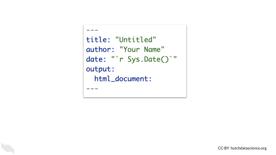
Here we can see what the top of an R Markdown file looks like after we first open one.

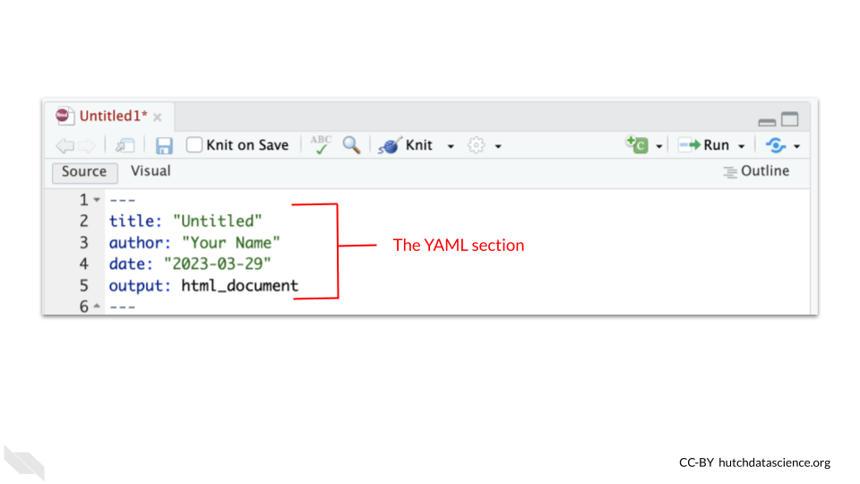
The YAML code at the top of R Markdown files sets up how the file will look and be rendered. Here we see that title specifies a title, author lists an author name, date will list a date, and output will specify how we want the file report to be rendered. The three dashed lines indicate the start and end of the YAML section.

You can modify the "Untitled" text after title: to specify the title of your report. If you want to change the author section where it says "your name" in the example if that was not by default want you wanted in your file.

5.4.2 Code chunks

Next as we scroll down, we will see gray section with some notation which is called a code “chunk”.

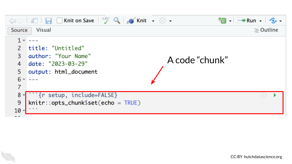
Image of a code chunk in the R Markdown file.

The notation here means the following:

The three back ticks "```" indicate the barriers of where some code will be in between. This is what we call an R chunk.
The {r} indicates that we are going to write the code using R code.
Extra information can be added inside the curly bracket {} notation to give the chunk a name, in this case it is called setup.
The include = FALSE means that it will not show up in the rendered report.

This first chunk tells the document how additional chunks should show up in the rendered report by default. Here it says that code should show up with echo = TRUE in the report. You don’t need to worry too much about any of this now, just recognize that this is a chunk of code.

As we scroll past some text within the R Markdown file, we will see another chunk.

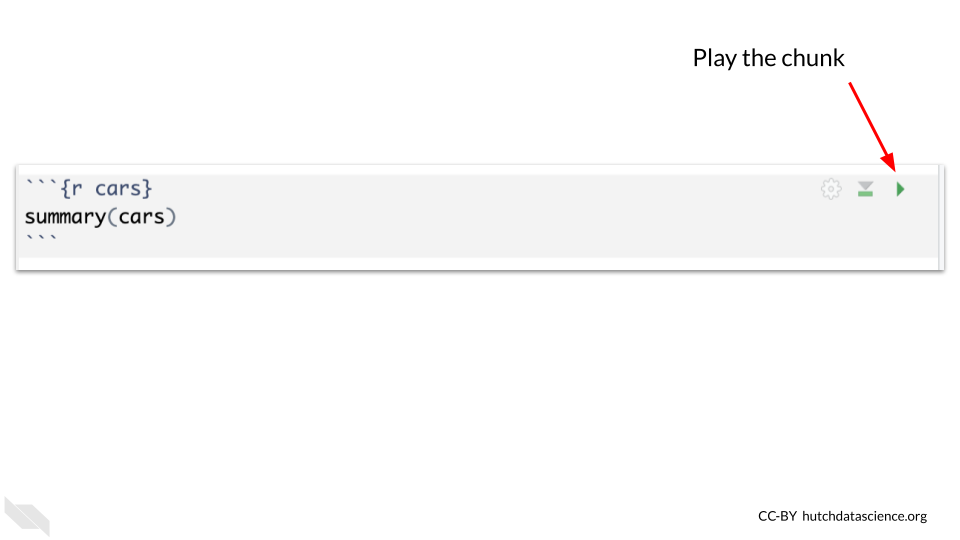
An image of the second R chunk in a new R Markdown file. Importantly there is a green play button that allows you to run the code within the chunk and see a preview of the output.

This chunk also has a name, “cars”. It is not necessary to name chunks, but it can help you to navigate to a particular chunk later, if you do name them.

5.4.3 Running chunks

Here we will see a green triangular button with its point facing to the right. This is the play button. If you try pressing this button inside of RStudio, you will see a preview of what the code does. It should show the summary of the cars data.

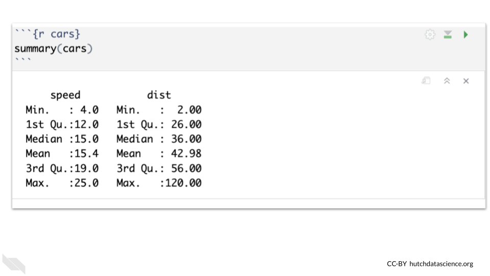
An image of what the code looks like after the play button is pressed for the second chunk.

Pretty nifty!

This is similar to testing our code in the console, in that if we assign an object it will show up in the environment.

Running a code chunk is like testing in the console, it will add any objects to the environment. Image shows that pressing the run button on a chunk that assigns data will create an object that shows up in the environment.

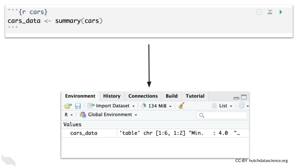
Code chunk - A piece of code in an R Markdown file. The code can be previewed pressing the play button for the chunk, which is equivalent to running the code in the console.

Writing our code in chunks (as opposed to one long script) can help with reproducibility, as we can better determine where possible changes may have occurred and how that influenced the results in a step-wise fashion, instead of just one final output.

5.4.4 Running previous chunks

You may also notice that there is another button to the left of the play button. This button allows you to play all previous chunks before this chunk.

An image of the second R chunk in a new R Markdown file. Importantly there is a play previous button that allows you to run the code within the chunks before this chunk.

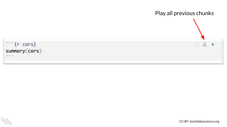
This is super helpful for reproducibility in terms of making sure that your code isn’t working simply because you have something in your environment from code that you tested in the console but did not save.

Issues can happen if you run a code chunk out of order or change the code in a chunk after running it previously. This can make you think that you have all the code that you need saved to obtain the result that you found, when in fact you do not.

Therefore we recommend cleaning the environment (which we will describe in the next section) and testing out that your chunks work well together by knitting the document. If you get an error you can run subsets of your code chunks together using the play previous button, until you identify where the issue occurred.

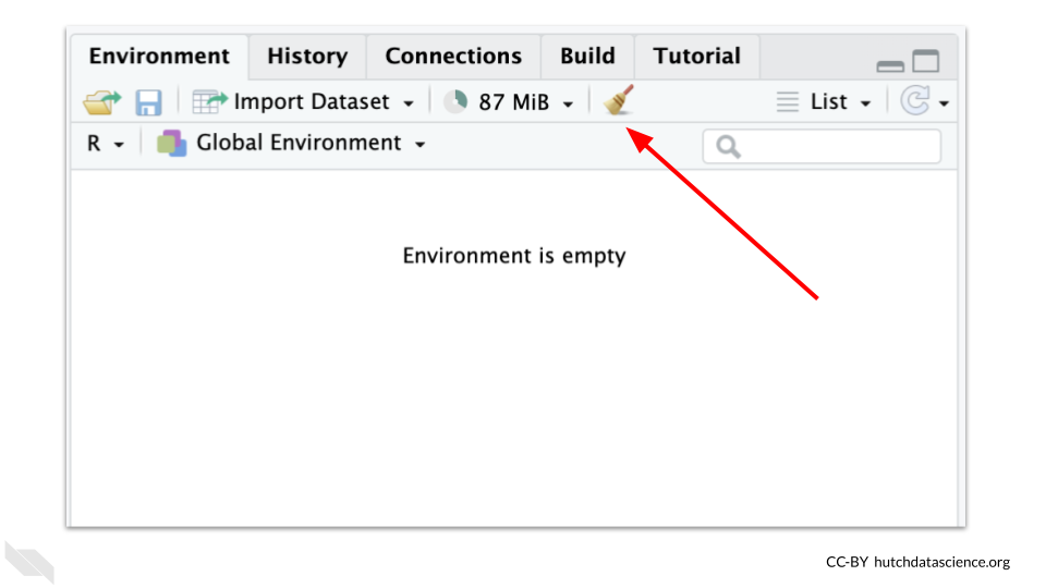
5.5 Cleaning the environment

We suggest cleaning out your environment somewhat regularly when you are interactively testing your R Markdown file using chunks. To do so, you can press the button that looks like a broom in the upper right pane.

Image showing the location of the broom button to clean the environment.

The ultimate test though is to press the Knit button and make sure you have all the code necessary to allow the report to render.

5.6 Restarting R Session

To really test your code, every once in a while, we suggest restarting your R Session and trying to Knit your R Markdown file to make sure that anything you loaded during your previous session (but didn’t save in your code) wasn’t allowing your code to run successfully.

To do so, you can click on the Session tab of the upper menu of RStudio and click Restart R.

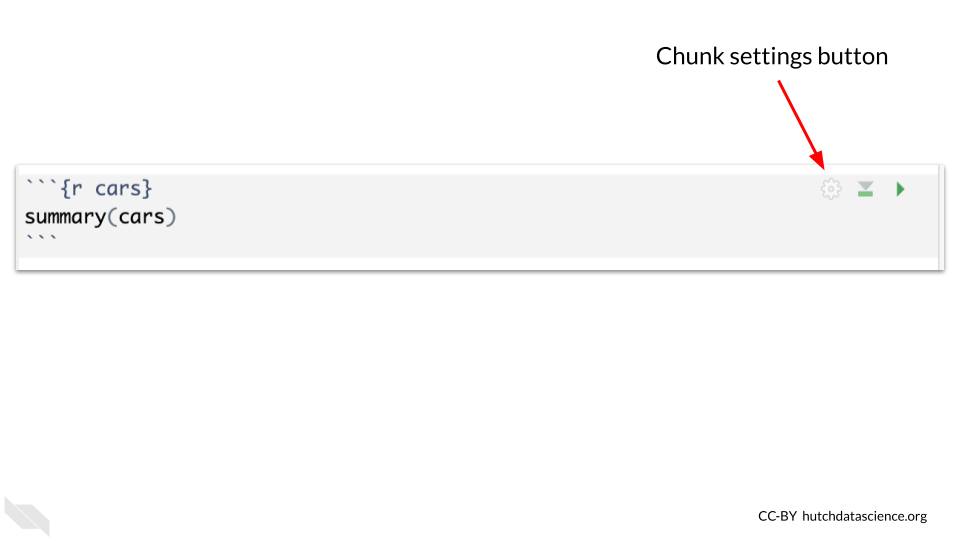
5.7 Chunk setup

You may find that sometimes you want to hide the code in a report, or hide the output. This can be for a variety of reasons. For example, the first chunk that is in every new R Markdown file (when you first open one) is hidden. This is because it sets up how all the other chunks work (by default) and it isn’t really important for the analysis. Recall that we hide the code and any output, using include = FALSE. If we just want to hide one or the other we can use different specifications.

The easiest way to do this is to click on the little gear symbol for the R chunk you wish to modify.

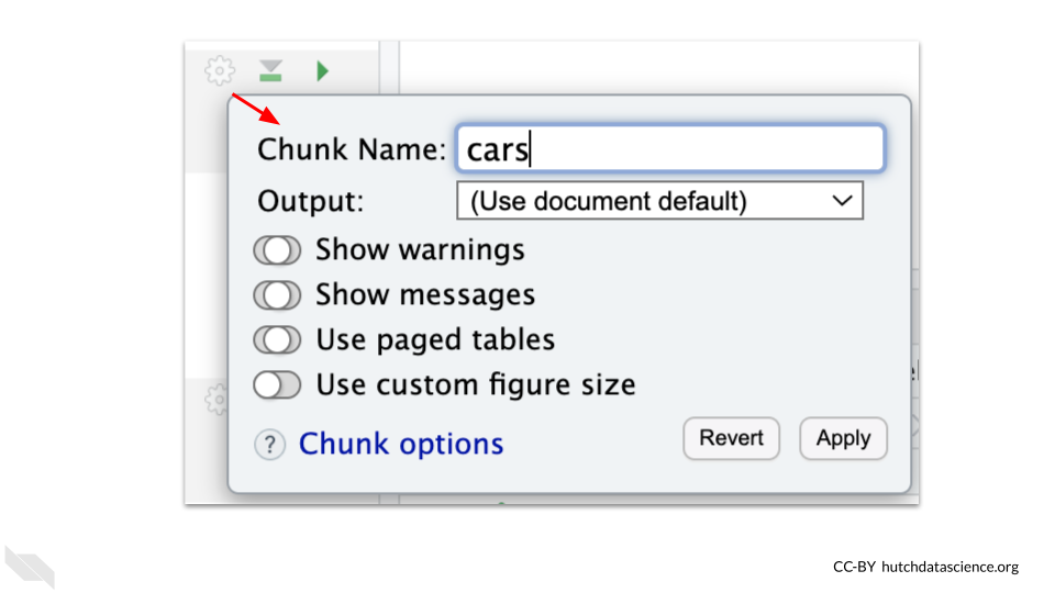
Image showing the gear button within a chunk.

This will open a menu about how that chunk should be set up. The dropdown menu can be used to select if you want the code to be hidden, the output to be hidden, both, or none to be hidden (the default).

Image of the chunk settings menu, where you can change the name of the chunk and use the pull down menu to change the output.

For reproducibility purposes, we generally suggest that you share the code, however, sometimes reports can get very difficult to read if you have all the code shown. So there are times where you might focus on a particular part of an analysis. We will also describe a nifty trick to allow readers of your report to see the code if they want to, but have it hidden most of the time.

5.8 Finding chunks

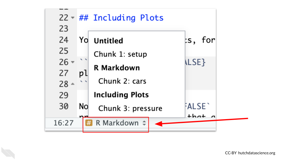
If your R Markdown file gets really long, it can be difficult to scroll to find the chunk you want to modify. If you name your chunks, or even if you don’t, you can more easily move around from one chunk to another using a special menu button created just for this!

There is a very small menu at the bottom of the R Markdown file editor that helps you move around. It will look slightly different depending on what your chunks are named, but will have a gold hashtag button.

The chunk search menu at the lower left corner of the R Markdown editor allows you to move form one chunk to another more easily.

5.9 Add chunks

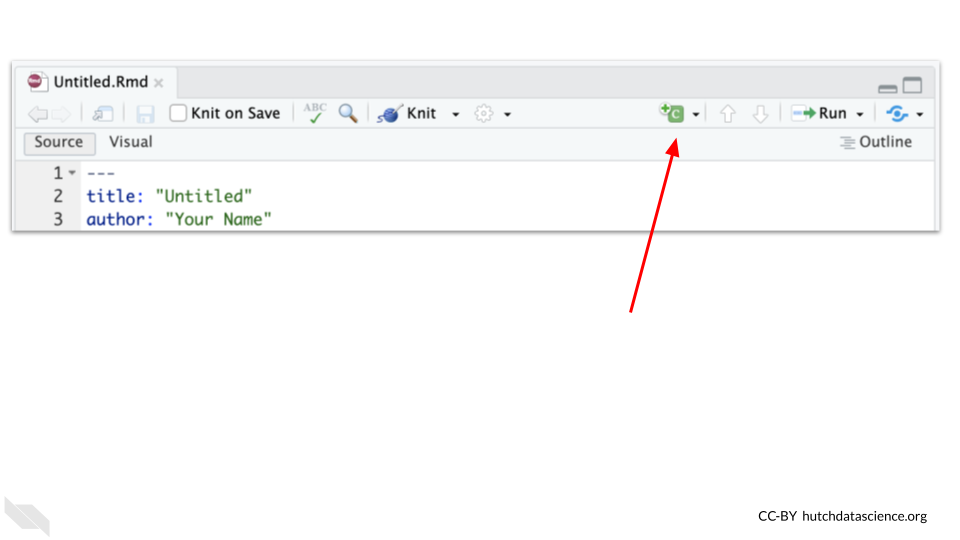
To add new chunks you can either click on the chunk button on the top right of the R Markdown editor, which looks like a green square with a “C” in it and a plus sign on the corner.

The button to add new chunks is located on the upper right corner of the R Markdown Editor. It looks like a green square with a C in it.

5.10 More on running chunks

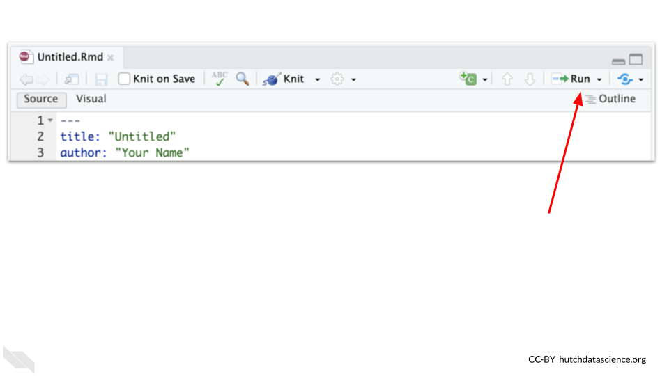
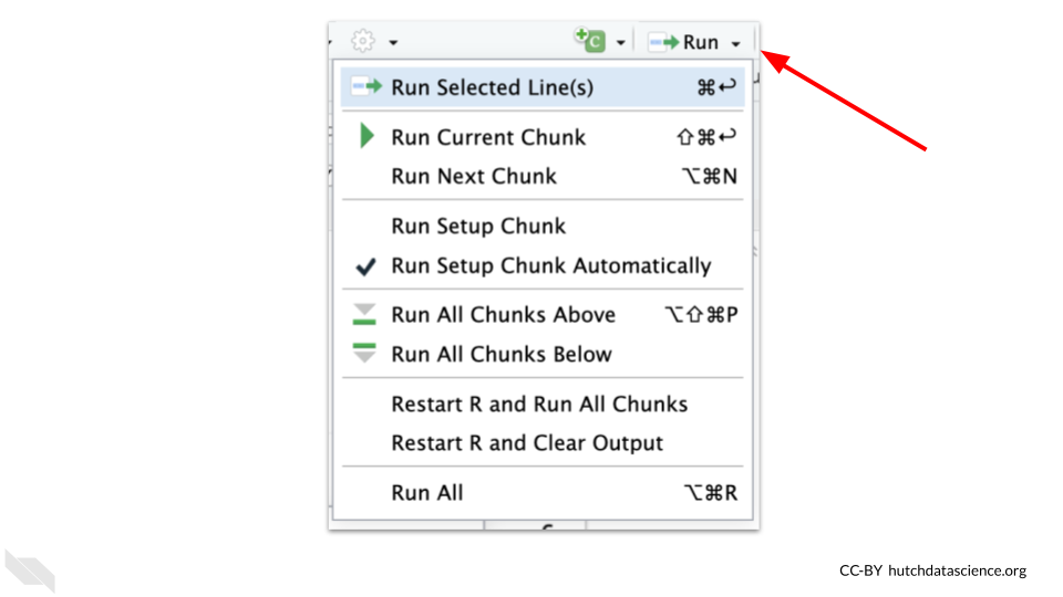
If you want to do anything fancier than running the current or previous chunks there is also a Run menu right next to the new chunk button. If you click on the arrow next to it, it will show you the advanced options. Otherwise it will just run all the chunks (which is similar to knitting but it will not render the report and may use objects that are in the environment).

The chunk run menu button is located to the right of the new chunk button.

The menu allows you to run all chunks below a specific chunk or run selected lines of code and more.

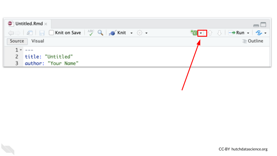
The chunk run menu allows you to run all chunks below a chunk.

The arrow next to the add chunk button, will allow you to specify if you want to use a different supported language besides R.

5.11 Text and headers

You will notice that there is text written around the code chunks that you can use to describe what you did in your analysis and why.

There are a couple of formatting options that can be very useful to know.

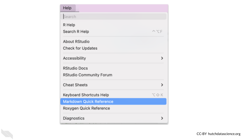
If you want to know more, you can check out this guide about Markdown in general. The syntax will be the same for R Markdown files too.

5.11.1 Headers

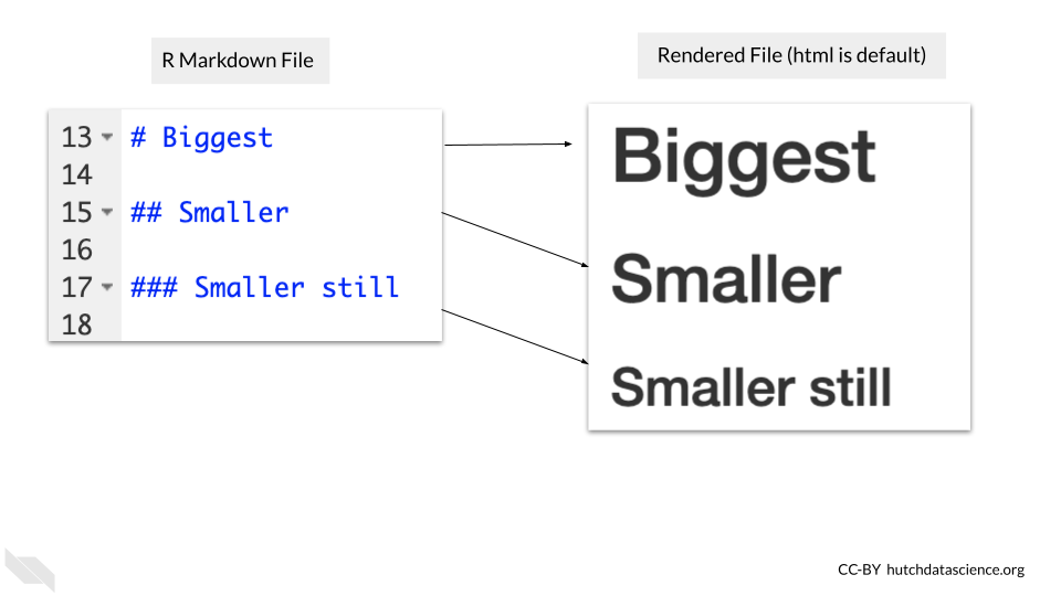
Using hashtags creates headers. One hashtag creates to highest level header, adding more hashtags add subsequent smaller headers. For example text with two ## will be smaller than text with one #. The hashtags need to be on the far right of the line and you need a space in between the hashtags and the text to create the header.

Adding one hashtag creates the top level header. Using additional hashtags creates smaller headers.

5.11.2 Bold and Italics

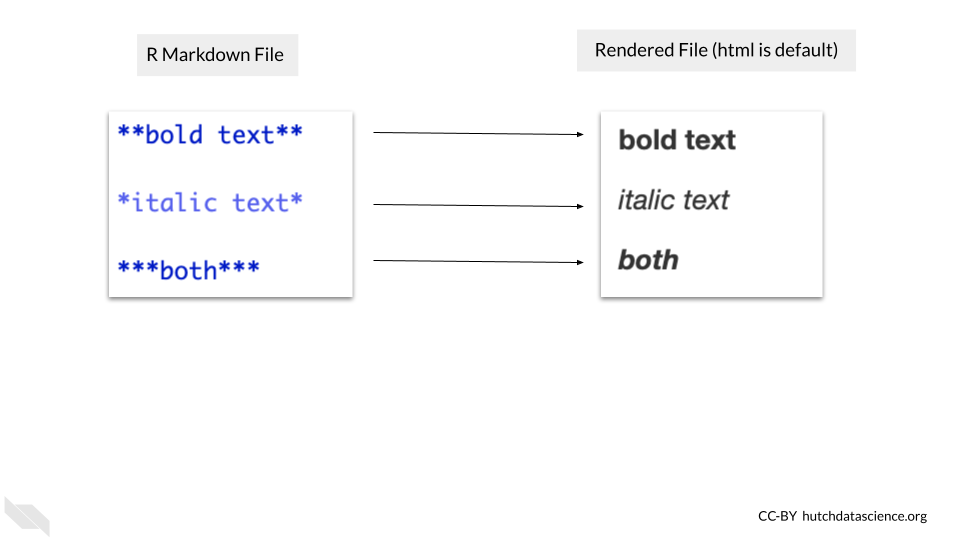
Bold text can be created using ** around the text.

Italic text can be created using * around the text.

To do both you can use *** around the text.

Using two asterisks around text creates bold text. Using one creates italic text. Using three creates text that is both bold and in italic.

The Help menu of RStudio has can open a markdown reference guide in the lower right pane under the help tab if you would like to learn more about writing text in R Markdown files.

The text surrounding our code and the output of our code can be extremely helpful in explaining to others what steps we took in our analysis, why we made certain decisions, the sources for our data and more. All of this information is extremely helpful for reproducibility!

5.12 Additional Features

We will cover a several additional features that we have found to be especially useful.

We also recommend checking out the R Markdown cookbook for even more tricks and tips.

5.12.1 Aesthetics

Sometimes we might want to make our reports look a little nicer, perhaps we want to add branding that matches that of our institute or at least makes the report look really polished.

You can make changes to the aesthetics of the report in very few steps.

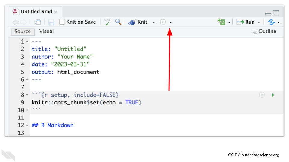
First locate the settings button for the R Markdown editor, which looks like a gear an is located next to the Knit button.

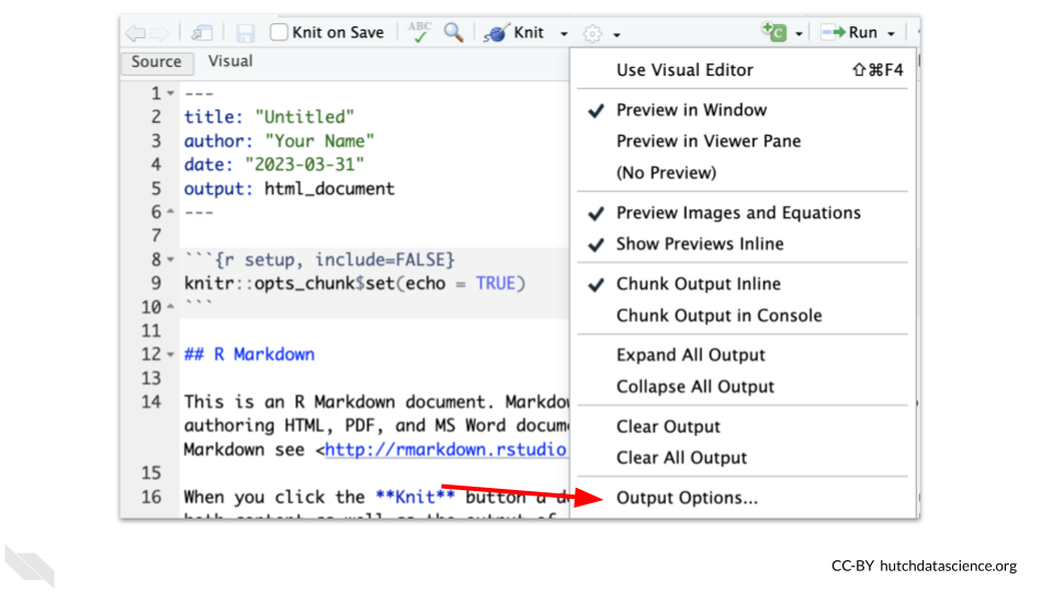
The R Markdown settings button is located to the right of the knit button. This opens a menu the helps you change the aesthetics of your rendered report.

Then scroll down and select “Output Options”. This menu also has nice features if you don’t like the default ways that the chunks preview output. For example, many people prefer to preview code in the console instead.

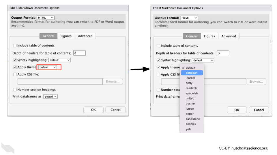
Scroll down to the Output Options to open the menu about aesthetics.

This will open a new window that has a dropdown that you can use to apply a theme to the report.

Use the dropdown menu next to the Apply theme section to change the theme of your R Markdown report.

This will modify the YAML code in your R Markdown file to add a line about the theme.

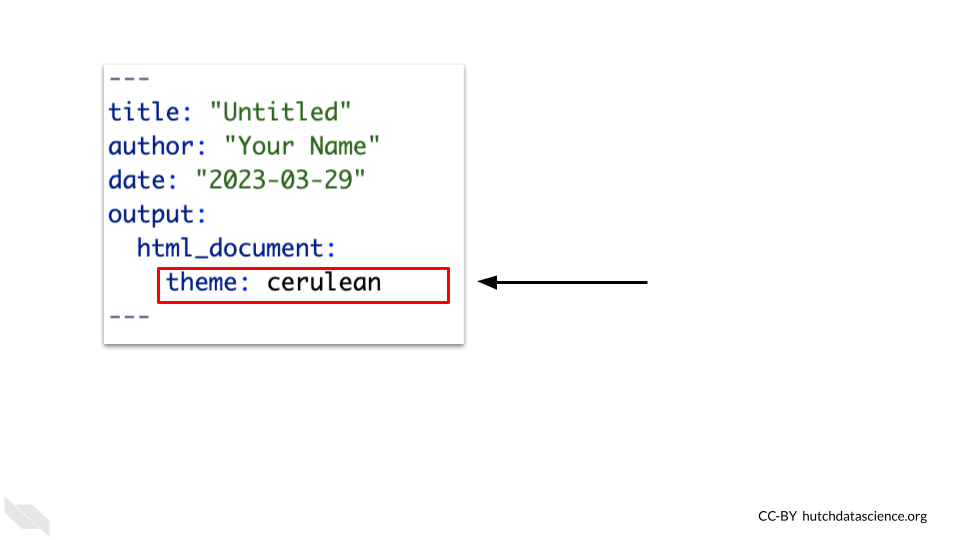
Selecting a different theme will modify the YAML code to change the way the report renders.

When the report is rendered it will have a different look.

The cerulean theme changes the way the report renders so that the fonts are different colors and more.

5.12.2 Report File Types

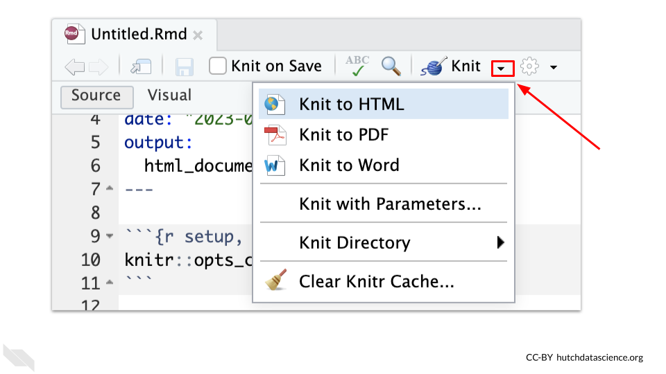
You can render your report as other file types besides html. This might be useful if a collaborator wants a PDF of your report. To do so click on the arrow next to knit button and select a different type. Here you can see that PDF and Word are other options. This will change the YAML code and may add more output information.

You can render your report as other file types besides html. To do so click on the arrow next to knit button and select a different type. Here you can see that PDF and Word are other options. This will change the YAML code and may add more output information.

5.13 Keyboard Shortcuts

If you like to work with keyboard shortcuts instead of pointing and clicking, you might also want to check out this link.

5.13.1 Table of Contents

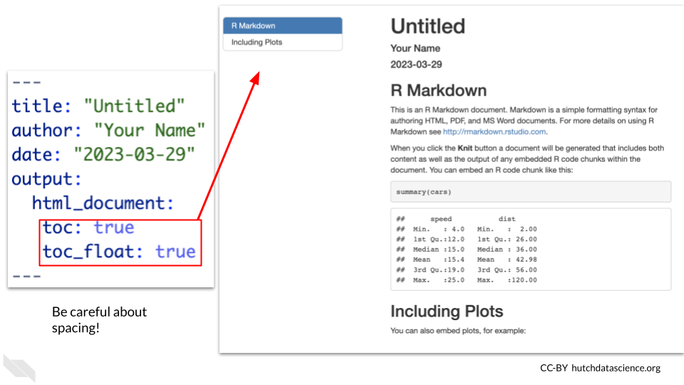
Sometimes if your report is very long, it can help to add a table of contents.

This can be done by adding toc: true and toc_float: true to the YAML underneath the html_document: code. The spacing is very important with this! The toc_float: true makes the table of contents on the side as opposed to just the top.

Modifying the YAML can add a table of contents to the R Markdown file report. Headings can be used to navigate.

5.13.2 Code Folding

Earlier we talked about hiding code but discussed that usually you want to share the code if possible. Code folding is really great option for this issue! It allows you to create a clean report with a button for people to click to see the code within the code chunk that resulted in the various outputs of the report.

To do this you can add code_folding: 'hide' to cause your code to be “folded”.

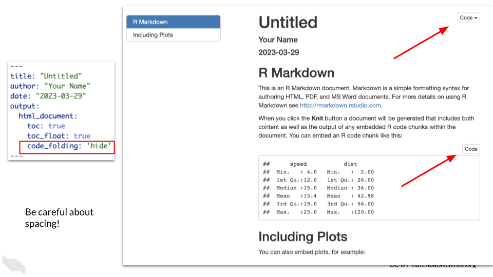
Modifying the YAML can allow for cold folding.

This means that there will be a button that people can click on to see the code (or hide it afterwards).

Code folding allows others to click on a code button to show the code, they can then click hide to hide it afterwards.

Cold Folding is a great option for reproducibility, because it makes your report easy to read, but also shares your code!

5.13.3 Code Download

You can allow others to download your code by adding code_download: true. The code button the top right will allow them to download the R Markdown file.

Be careful about allowing this if you use code that works with data with PHI. Just make sure that no PHI would be described in the R Markdown file itself as opposed to the rendered report.

5.13.4 Automatic Date

Using date: "2023-04-28" in the YAML will keep the date up-to-date as you write more code. It will display the date that the report was last rendered.

Modifying the YAML make it so the date updates to whatever day the report was last rendered

This trick is great for reproducibility because it ensures that the date on the report is correct for when the report was last rendered. This helps those who read the report to get a sense of how active development is on the project.

5.14 Conclusion

In summary, R Markdown files can help you to create nice looking reports that help others to understand not only what code you used, but also what the results of your code were.

Code is written in gray sections called chunks that have play buttons that allow you to preview the code
The Knit button allows you to render the full report and test that all of the needed code is in the file
Using the Knit button does not rely on anything in the environment, all objects needed or any data that needs to be imported must be done within the R Markdown file code
New chunks can be added using the new code chunk button which looks like a green square with a “C” in it at the top of the R Markdown editor
Chunks can be set up to hide the code, or the output, or hide both, or hide neither (the default)
The gear button on each chunk can be used to set the output for a given chunk
The play previous button to the left of the play button will run the code for all previous chunks
To make sure that you are not relying on code that was just run in the console or run by playing a chunk, it is advisable to clean the environment with the broom button from time to time
hashtags are used to create headers, the fewer the hashtags the larger the header
Asterisk around text creates bold or italic font
There are additional features to make your R Markdown report showcase your code and the output of your code in more readable ways, including adding a table of contents or folding code, so that readers can click to see the code that created a particular output. This is a really great option for reproducibility because it creates easy to read reports but also shares your code!