Part I: Analyses of software infrastructure

This analysis aims to explore the software infrastructure of 44 tools (33 funded by ITCR alone and 7 funded by the Cancer Target Discovery and Development (CTD²) Network, as well as 4 tools funded by both) and provide insights into their trends, documentation, dependencies, and citation metrics.

# Read data and recode
wdat <- read_csv(file = "tooldata_anonymized.csv") 

## Recode the health_metrics into simple classification
wdat %<>% 
  mutate(simple_health_metrics = case_when(
    str_detect(health_metrics, "no|No|unknown status|no badge|Not for core software|CI but not badge|\\?") ~ "No",
    str_detect(health_metrics, "Yes|yes|Test badges|CI and coverage badges|bioconductor only| with badge") ~ "Yes",
    TRUE ~ health_metrics))

## Recode type of data into simple classification

wdat %<>% 
  mutate(dataType = case_when(
    str_detect(`type of data`, "DNA methylation and gene expression|Gene sets|genomics|methylation|microbiome sequence analysis|mostly proteomics|multi-omics|mutation analysis|phenotypic associations|protein-protein interaction networks|genomic, phenotypic") ~ "Omics",
    str_detect(`type of data`, "cancer models|clinical study metadata harmonization|clinical text") ~ "Clinical",
    str_detect(`type of data`, "digital pathology slides|Imaging|PET/CT image analysis|image analysis") ~ "Imaging",
    str_detect(`type of data`, "multi-omics|mixed|genomic|Analysis of Variants") ~ "Multiple Data Types",
    TRUE ~ `type of data`))

## Recode type of tool into simple classification

#wdat %>% count(toolType)

wdat %<>% rename(toolType = `class/type`) %>% 
  mutate(
    toolType = case_when(
      str_detect(toolType, "Suite") ~ "Suite",
      str_detect(toolType, "Platform") ~ "Computing Platforms",
      str_detect(toolType, "Command-line tool/Other scripts|Desktop Application") ~ "Desktop Applications/\nCommand-line tools",
      str_detect(toolType, "Web") ~ "Web-based Tools",
      str_detect(toolType, "Jupyter|Python") ~ "Jupyter/Python",
      str_detect(toolType, "R") ~ "R-packages",
      TRUE ~ toolType
    )
  )

Graphical Analyses

We have made use of color-blindness friendly colors in our analyses.

1. Distribution of software across tool and data types

toolsPlot <- wdat %>% 
  ggplot(aes(x = fct_infreq(toolType), fill = toolType)) +
  geom_bar(width = 0.5) +
  geom_text(stat = 'count', 
            aes(label = paste0(after_stat(round(100*count/sum(count),1)), "%")), 
            hjust = 1.5, color = "white") +
  labs(x = "", y = "Frequency", 
       caption = "Distribution of Software Across Tool Types") +
  scale_y_continuous(n.breaks = 10) +
  scale_fill_manual(values = c("#E69F00", "#89B4E9", "#0Fadff", "#009E7A", "#D55E00", "#0072B2", "#CC79A7")) +
  ggtitle("Software Tool Types") +
  theme_light() +
  theme(axis.text.x = element_text( vjust = 0.5, hjust = 1),
        axis.text.y = element_text(size = 10),
        axis.title.y = element_text(angle = 0, vjust = 1, size = 12),
        panel.grid.major = element_line(color = "#ffffff"),
        panel.grid.minor = element_blank(),
        legend.position = "none") + coord_flip()

toolsPlot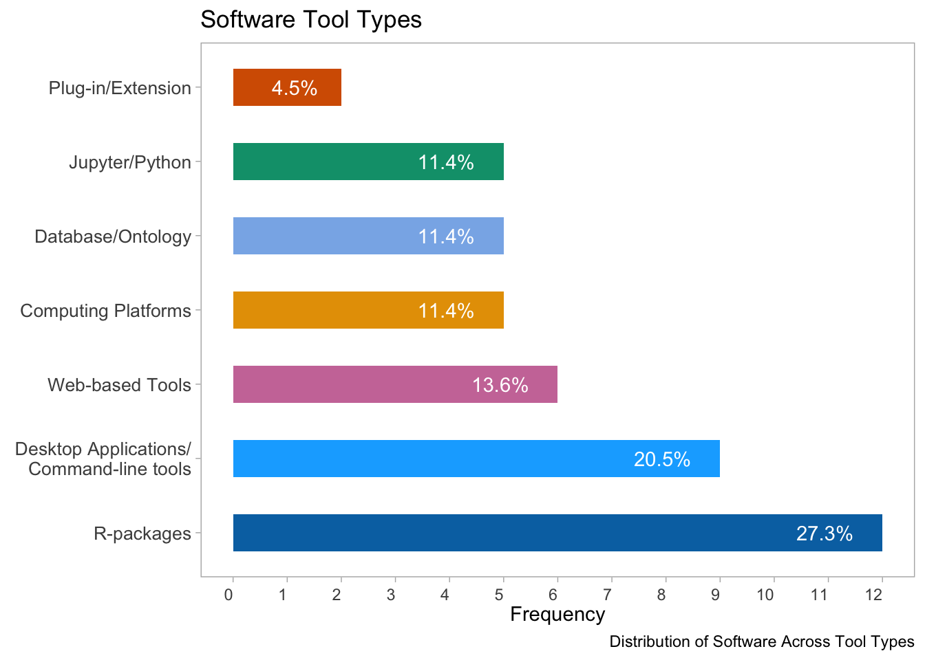

ggsave("software_tool_types.png", plot = toolsPlot, dpi = 300, width = 8, height = 6, units = "in")

The vertical bar plot shows the distribution of software across different tool types. The x-axis represents the frequency of the software and is labeled with the tool types. The y-axis represents the frequency of occurrence of the software. Each tool type is represented by a different color. The percentage of each tool type is displayed on top of the corresponding bar.
The majority of the users use R-packages, and Desktop Applications or Commandline tools, while a few use computing platforms, Jupyter/Python, Database/Ontology, and Plug-in/Extension.

wdat %>%
  ggplot(aes(x = fct_infreq(dataType), fill = dataType)) +
  geom_bar(width = 0.5) +
  geom_text(stat = 'count', 
            aes(label = paste0(after_stat(round(100*count/sum(count),1)), "%")), 
            hjust = 1.1, color = "white") +
  labs(x = "", y = "Frequency", 
       caption = "Distribution of Software Across Data Types") +
  scale_y_continuous(n.breaks = 13) +
  scale_fill_manual(values = c("#E69F00", "#56B4E9", "#009E73", "#0072B2", "#D55E00", "#CC79A7")) +
  ggtitle("Software Data Types") +
  theme_light() +
  theme(axis.text.x = element_text( vjust = 0.5, hjust = 1),
        axis.text.y = element_text(size = 10),
        axis.title.y = element_text(angle = 0, vjust = 1, size = 12),
        panel.grid.major.y = element_line(color = "#ffffff"),
        panel.grid = element_blank(),
        legend.position = "none") + 
  coord_flip()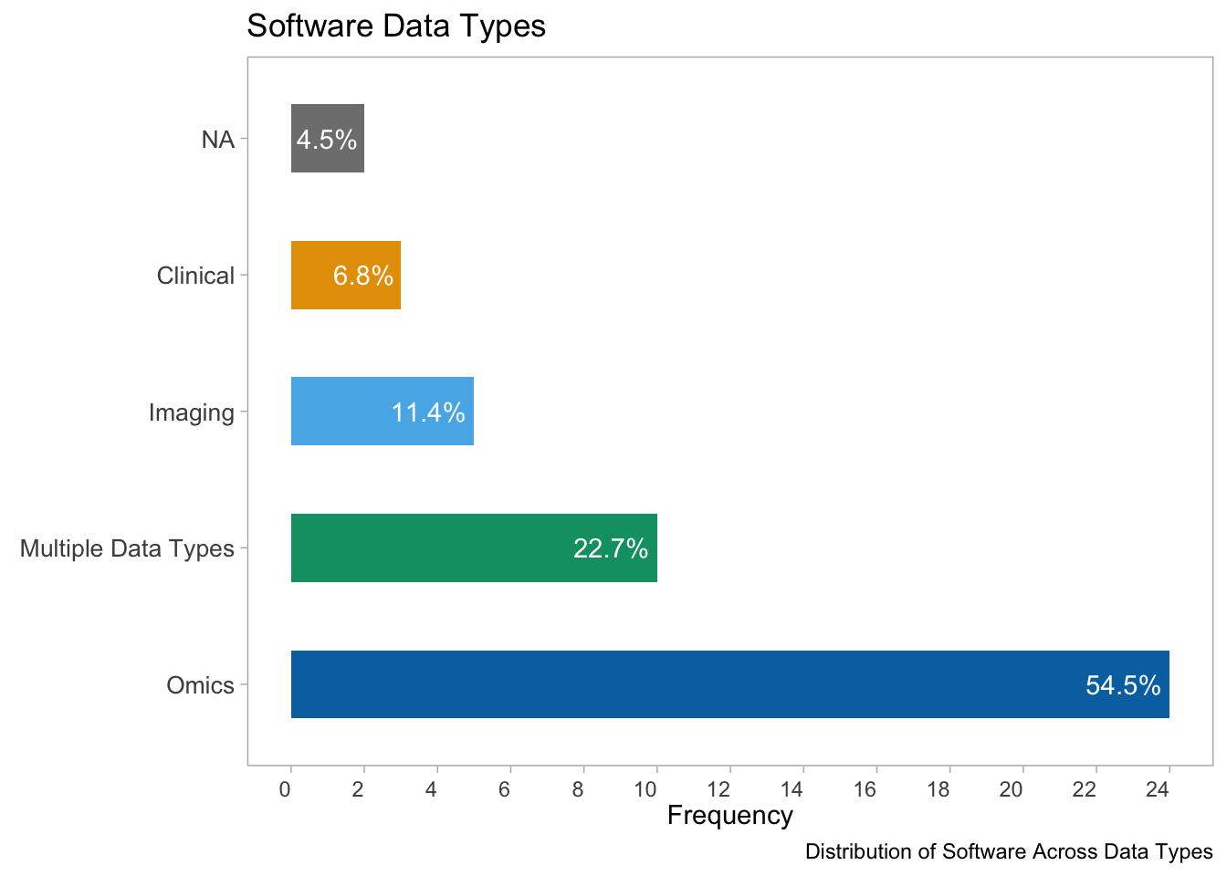

This plot shows the distribution of software across different data types. The x-axis represents the frequency of each data type, and the bars are color-coded by data type. The various omics-data type is the most frequently used data for the software platforms.

2. Distribution of software having simple health metrics

Here we look at the distribution of software having simple health metrics (Test badges, CI and coverage badges etc.):
Note: the category “NA” refers to the that the particular tool did not have any repository or website that allows observation of such tags/metrics.
CI stands for Continuous Integration (regularly merging code changes into a central repository, after which automated builds and tests are run.)

wdat %>% mutate(simple_health_metrics = if_else(is.na(simple_health_metrics), "NA", simple_health_metrics)) %>% 
  ggplot(aes(x = simple_health_metrics, fill = simple_health_metrics)) +
  geom_bar( width = 0.5, show.legend = F) + 
  geom_text(stat = 'count', 
            aes(label = paste0(after_stat(round(100*count/sum(count),1)), "%")), vjust = 1.5, color = "white") +
  labs(x = "simple health metrics", y = "Frequency", fill = "simple \nhealth metrics",
       caption = "Distribution of software with simple health metrics") +
  scale_y_continuous(n.breaks = 10) + 
    scale_fill_manual(values = c("gray50", "#CC79A7", "#009E73")) +
  theme_light() +
  theme(panel.grid = element_blank())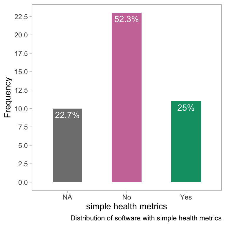

The bar plot shows the distribution of software based on the presence of simple health metrics such as test badges, coverage badges, and CI badges. The x-axis shows the simple health metrics while the y-axis shows the frequency of the software. The plot suggests that most software does not have any simple health metrics, followed by software with test badges, and then software with coverage badges.

wdat %>% mutate(simple_health_metrics = if_else(is.na(simple_health_metrics), "NA", simple_health_metrics)) %>% 
  ggplot(aes(x = fct_infreq(simple_health_metrics), fill = simple_health_metrics)) +
  geom_bar( width = 0.5) + 
  facet_wrap(~toolType, ncol = 3) +
  geom_text(stat = 'count', aes(label = after_stat(count), vjust = 1.2), color = "white") +
  labs(x = "simple health metrics", y = "Frequency", fill = "Simple \nhealth metrics",
       caption = "Distribution of software with simple health metrics across tool types") +
  scale_y_continuous(n.breaks = 10) + 
  scale_fill_manual(values = c("gray50", "#CC79A7", "#009E73")) +
  theme_light() +
  theme(strip.background = element_rect(fill = "steelblue4"),
        strip.text = element_text(colour = 'white', size = 11),
        panel.grid = element_blank())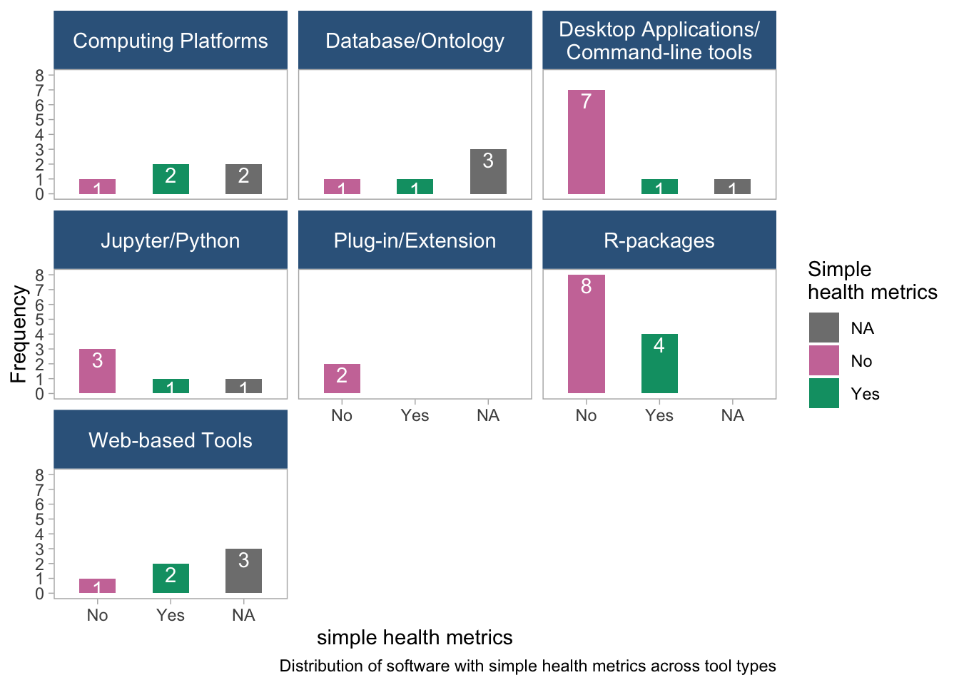

The plot is faceted by tool type and suggests and highlights the difference in the distribution of simple health metrics across tool types.

wdat %>% mutate(simple_health_metrics = if_else(is.na(simple_health_metrics), "NA", simple_health_metrics)) %>% 
  ggplot(aes(x = fct_infreq(simple_health_metrics), fill = simple_health_metrics)) +
  geom_bar( width = 0.5) + 
  facet_wrap(~dataType) +
  geom_text(stat = 'count', aes(label = after_stat(count), vjust = 1.2), color = "white") +
  labs(x = "simple health metrics", y = "Frequency", fill = "Simple \nhealth metrics",
       caption = "Distribution of software with simple health metrics across data types") +
  scale_y_continuous(n.breaks = 10) + 
  scale_fill_manual(values = c("gray50", "#CC79A7", "#009E73")) +
  theme_light() +
  theme(strip.background =element_rect(fill="steelblue4"),
        strip.text = element_text(colour = 'white', size = 11), 
        panel.grid = element_blank())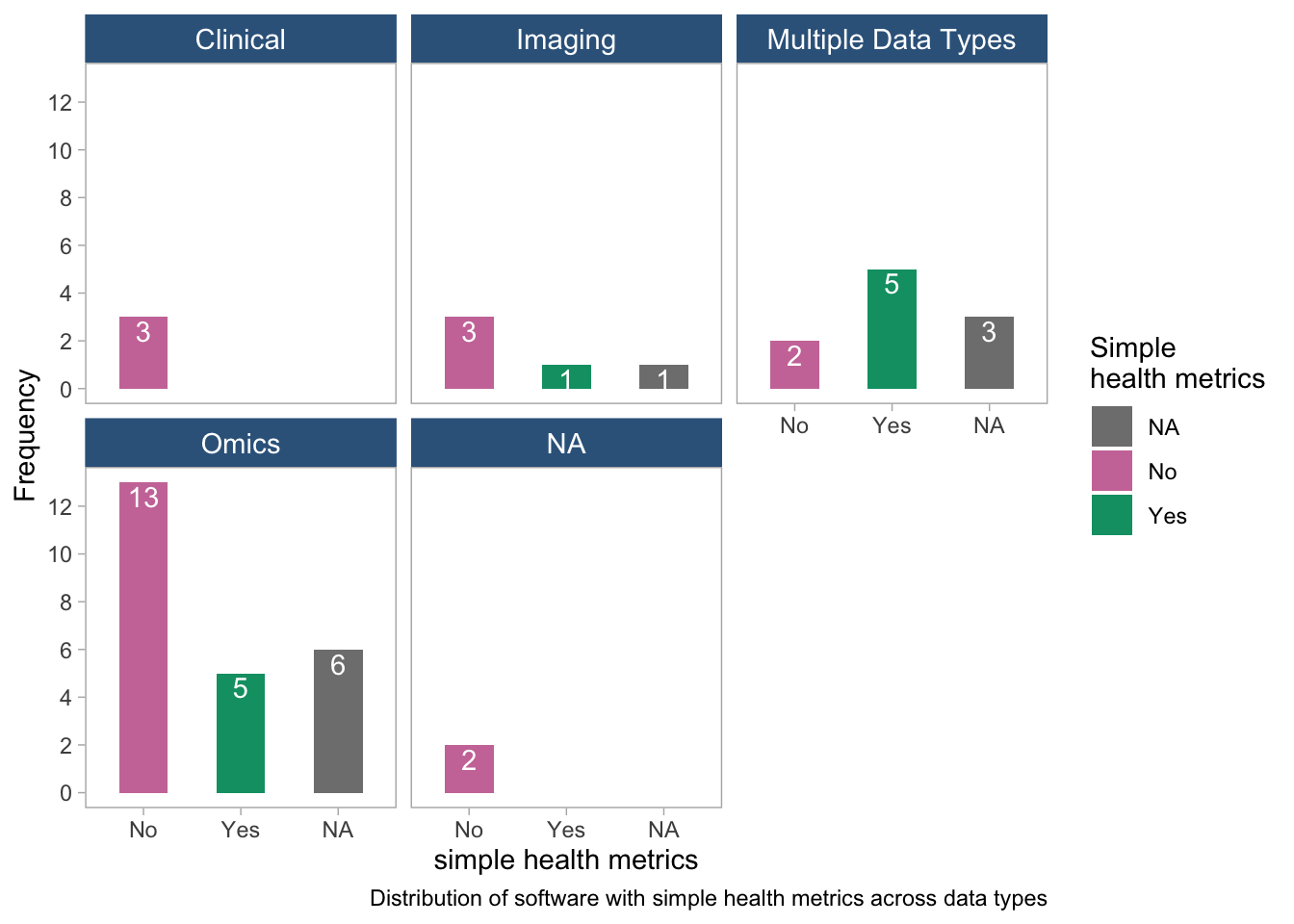

The plot suggests that clinical software do not have any simple health metric. The distribution of software with simple health metrics is high for multiple data types.

3. Distribution of software having their own DOI

Here we look at the distribution of software having their own DOI (digital object identifier):

wdat %>% 
  ggplot(aes(x = fct_infreq(ownDOI), fill = ownDOI)) +
  geom_bar( width = 0.5, show.legend = F) + 
  geom_text(stat = 'count', aes(label = paste0(after_stat(round(100*count/sum(count),1)), "%")), vjust = 1.5, color = "white") +
  labs(x = "software with DOI", y = "Frequency", caption = "Distribution of software with own DOI") +
  scale_y_continuous(n.breaks = 10) + 
   scale_fill_manual(values = c("#CC79A7", "#009E73")) +
  theme_light() +
  theme(panel.grid = element_blank())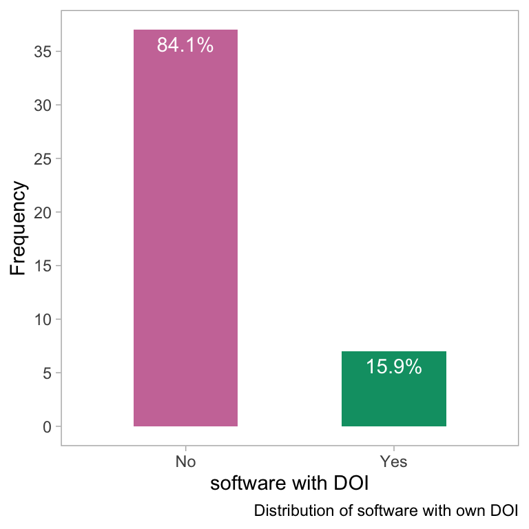

The bar plot shows the distribution of software based on the presence of a digital object identifier (DOI). The plot suggests that the majority of software do not have its own DOI, while a small portion of software does have one.

wdat %>% 
  ggplot(aes(x = ownDOI, fill = ownDOI)) +
  geom_bar( width = 0.5, show.legend = F) + 
  geom_text(stat = 'count', aes(label = after_stat(count), vjust = 1.5), color = "white") +
  facet_wrap(~toolType) +
  labs(x = "softwares with DOI", y = "Frequency", caption = "Distribution of softwares with own DOI across tool types") +
  scale_y_continuous(n.breaks = 10) + 
   scale_fill_manual(values = c("#CC79A7", "#009E73")) +
  theme_light() +
  theme(strip.background =element_rect(fill="steelblue4"),
        strip.text = element_text(colour = 'white', size = 11),
        panel.grid = element_blank())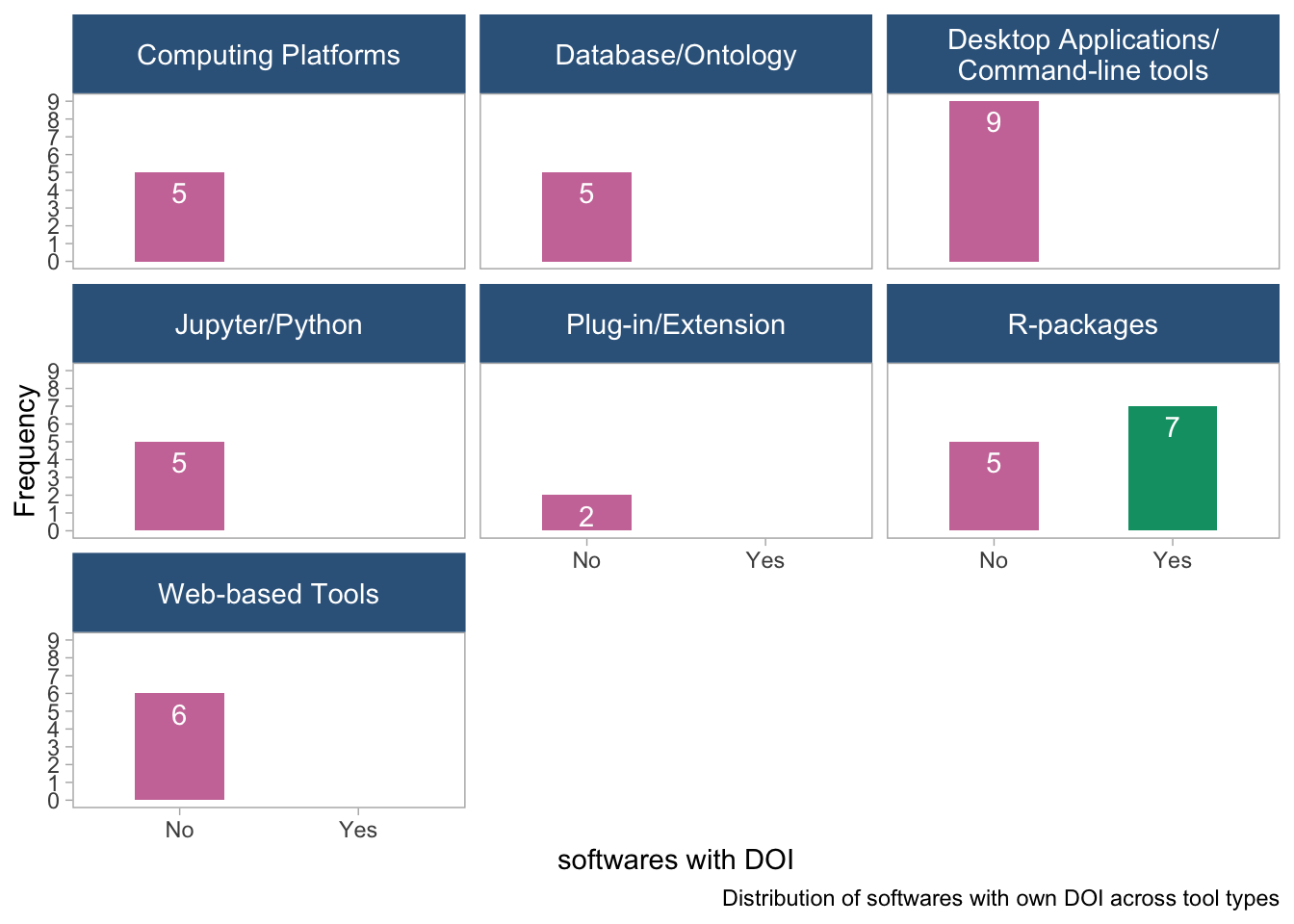

Only the R-packages (Bioconductor and others) have DOI available. The other software types do not.

4. Distribution of Twitter presence

## Marginal dist
wdat %>% 
  ggplot(aes(x = socialMedia, fill = fct_infreq(socialMedia))) + 
  geom_bar(position = "dodge", width = .6, show.legend = F) + 
  geom_text(stat = 'count', color = "white",
            aes(label = paste0(after_stat(round(100*count/sum(count),1)), "%")), position = position_dodge(width = .9), vjust = 1.5) +
  labs(x = "Twitter Presence", y = "Frequency", fill = "Twitter Presence", caption = "Distribution of Twitter Presence") +
  scale_y_continuous(n.breaks = 7) + 
  scale_fill_manual(values = c("#CC79A7", "#009E73")) +
  theme_light()  +
  theme(panel.grid = element_blank())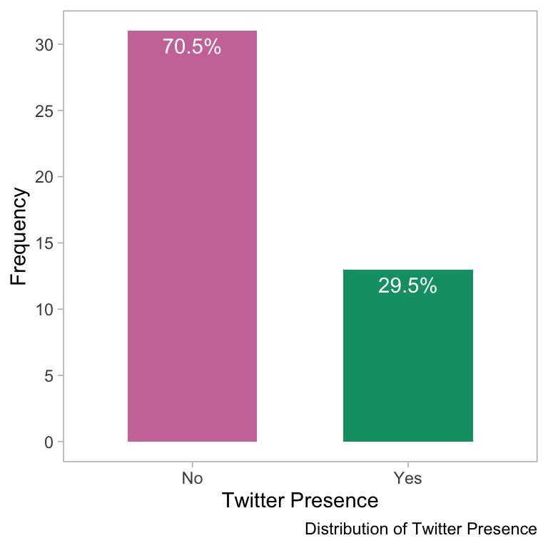

The bar plot shows the distribution of Twitter presence among the software tools. The x-axis represents the presence or absence of a Twitter account, and the y-axis shows the frequency of the software. The majority of software tools do not have a Twitter presence and only 30% of the tools have a Twitter presence.

## Stratified by tool type
wdat %>% 
  ggplot(aes(x = socialMedia, fill = fct_infreq(socialMedia))) + 
  geom_bar(position = "dodge", width = .6, show.legend = F) + 
  geom_text(stat = 'count', color = "white",
            aes(label = paste0(after_stat(count))), position = position_dodge(width = .9), vjust = 1.2) +
  facet_wrap(~toolType) +
  labs(x = "Twitter Presence", y = "Frequency", fill = "Twitter Presence", caption = "Distribution of Twitter Presence") +
  scale_y_continuous(n.breaks = 7) + 
  scale_fill_manual(values = c("#CC79A7", "#009E73")) +
  theme_light() + 
  theme(strip.background =element_rect(fill="steelblue4"),
        strip.text = element_text(colour = 'white', size = 11),
        panel.grid = element_blank())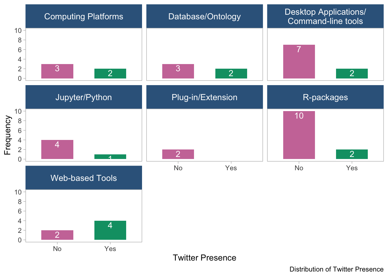

This bar plot, stratified by tool type, also shows the distribution of Twitter presence among the software tools. The plots suggest that there are variations in the distribution of Twitter presence across different tool types.

## Stratified by data type
wdat %>% 
  ggplot(aes(x = socialMedia, fill = fct_infreq(socialMedia))) + 
  geom_bar(position = "dodge", width = .6, show.legend = F) + 
  geom_text(stat = 'count', color = "white",
            aes(label = paste0(after_stat(count))), position = position_dodge(width = .9), vjust = 1.1) +
  facet_wrap(~dataType) +
  labs(x = "Twitter Presence", y = "Frequency", fill = "Twitter Presence", caption = "Distribution of Twitter Presence across data types") +
  scale_y_continuous(n.breaks = 7) + 
  scale_fill_manual(values = c("#CC79A7", "#009E73")) +
  theme_light() + 
  theme(strip.background =element_rect(fill="steelblue4"),
        strip.text = element_text(colour = 'white', size = 11),
        panel.grid = element_blank())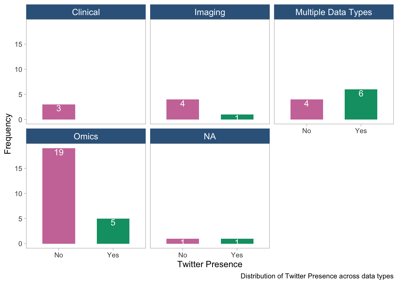

The bar plot shows the distribution of Twitter presence across data types. The plot suggests that most data types do not have Twitter presence, except those with multiple data types. However the overall frequency in Clinical and Imaging types are too low to draw conclusions.

5. Distribution of presence of instruction on How to Cite

wdat %>% 
  ggplot(aes(x = fct_infreq(citeHow), fill = citeHow)) +
  geom_bar(position = "dodge", width = .5, show.legend = F) + 
  geom_text(stat = 'count', color = "white",
            aes(label = paste0(after_stat(round(100*count/sum(count),1)), "%")), position = position_dodge(width = .9), vjust = 1.5) +
  labs(x = "Instruction availability on How to Cite", y = "Frequency", caption = "Distribution of Citation Instructions") +
  scale_y_continuous(n.breaks = 12) + 
  scale_fill_manual(values = c("#CC79A7", "grey50", "#009E73")) +
  theme_light() +
  theme(panel.grid = element_blank())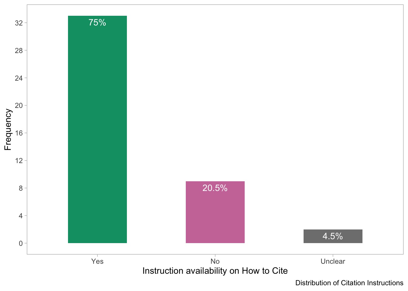

The bar plot shows the distribution of software based on the presence of instructions on how to cite it. The x-axis shows the availability of citation instructions while the y-axis shows the frequency of the software. The plot suggests that the majority of software provides instructions on how to cite it,

## Stratified  by toolType
wdat %>% 
  ggplot(aes(x = fct_infreq(citeHow), fill = citeHow)) +
  geom_bar(position = "dodge", width = .5, show.legend = F) + 
  geom_text(stat = 'count', color = "white",
            aes(label = paste0(after_stat(count))), position = position_dodge(width = .9), vjust = 1.2) +
  facet_wrap(~toolType) +
  labs(x = "Instruction availability on How to Cite", y = "Frequency", caption = "Distribution of Citation Instructions") +
  scale_fill_manual(values = c("#CC79A7", "grey50", "#009E73")) +
  theme_light() +
  theme(strip.background =element_rect(fill="steelblue4"),
        strip.text = element_text(colour = 'white', size = 11),
        panel.grid = element_blank())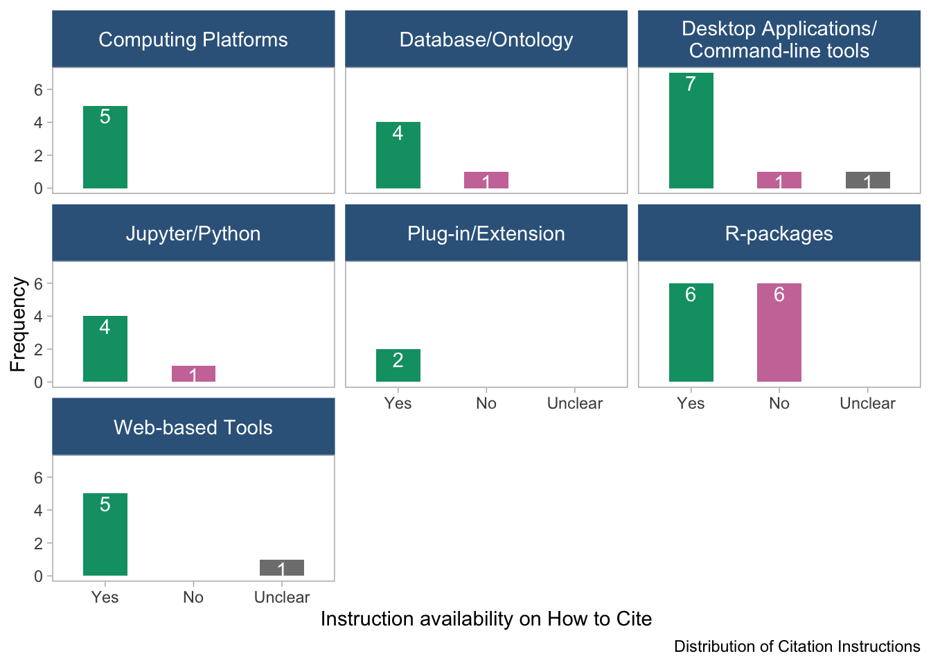

It appears that the half of the R-packages do not provide instruction on how to cite them.
“NA” refers to tools with unavailable information on data type.

## Stratified  by dataType
wdat %>% 
  ggplot(aes(x = fct_infreq(citeHow), fill = citeHow)) +
  geom_bar(position = "dodge", width = .5, show.legend = F) + 
  geom_text(stat = 'count', color = "white",
            aes(label = paste0(after_stat(count))), position = position_dodge(width = .9), vjust = 1.2) +
  facet_wrap(~dataType) +
  labs(x = "Instruction availability on How to Cite", y = "Frequency", caption = "Distribution of Citation Instructions") +
  scale_fill_manual(values = c("#CC79A7", "grey60", "#009E73")) +
  theme_light() +
  theme(strip.background =element_rect(fill="steelblue4"),
        strip.text = element_text(colour = 'white', size = 11),
        panel.grid = element_blank())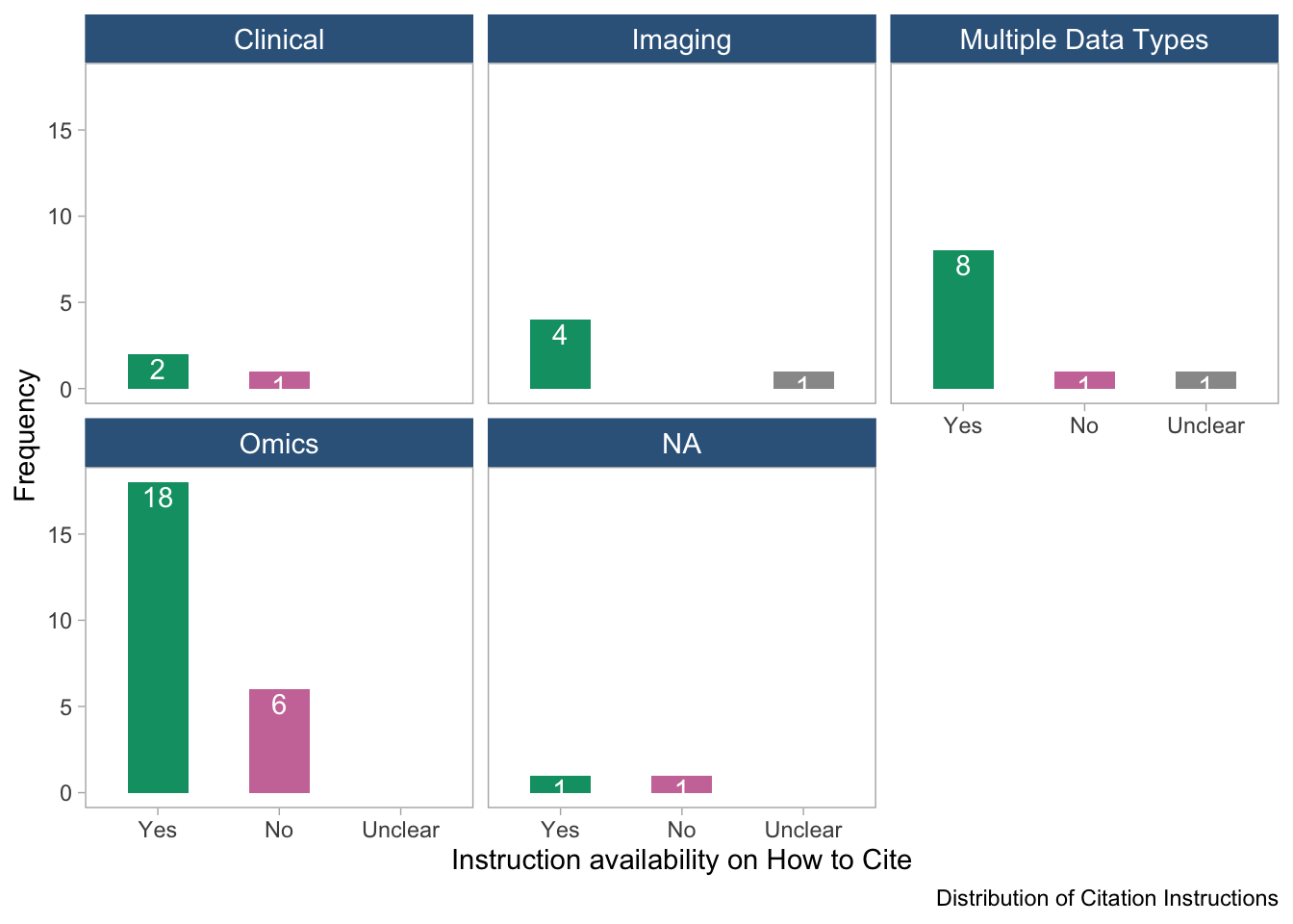

The bar plot shows the distribution of citation instructions across data types.

6. Age distribution of the tool

## Tool Age distribution
age1 <- wdat %>% select(releaseYear) %>% mutate(releaseYear = as.factor(releaseYear)) %>% 
  ggplot(aes(x = releaseYear, fill = releaseYear)) +
  geom_bar(position = "dodge", width = .5, show.legend = F) + 
  labs(x = "Release Year", y = "Frequency", caption = "Distribution of Tool releases across the years") +
  scale_y_continuous(n.breaks = 7) + 
  #scale_fill_brewer(palette = "Set3", direction = 1) +
  theme_light() +
  theme(panel.grid.minor = element_blank())

age2 <- wdat %>%
  ggplot(aes(x = toolAge)) +
  geom_histogram(aes(y = after_stat(density)), fill = "white", col = "darkgray", binwidth = 2) +
  geom_density(col = "steelblue2") +
  scale_x_continuous(breaks = seq(0, 22, by = 2)) +
  labs(x = "Tool Age", y = "Density", subtitle = "Tool Age distribution") +
  theme_light() + 
  theme(panel.grid = element_blank())

age1/ age2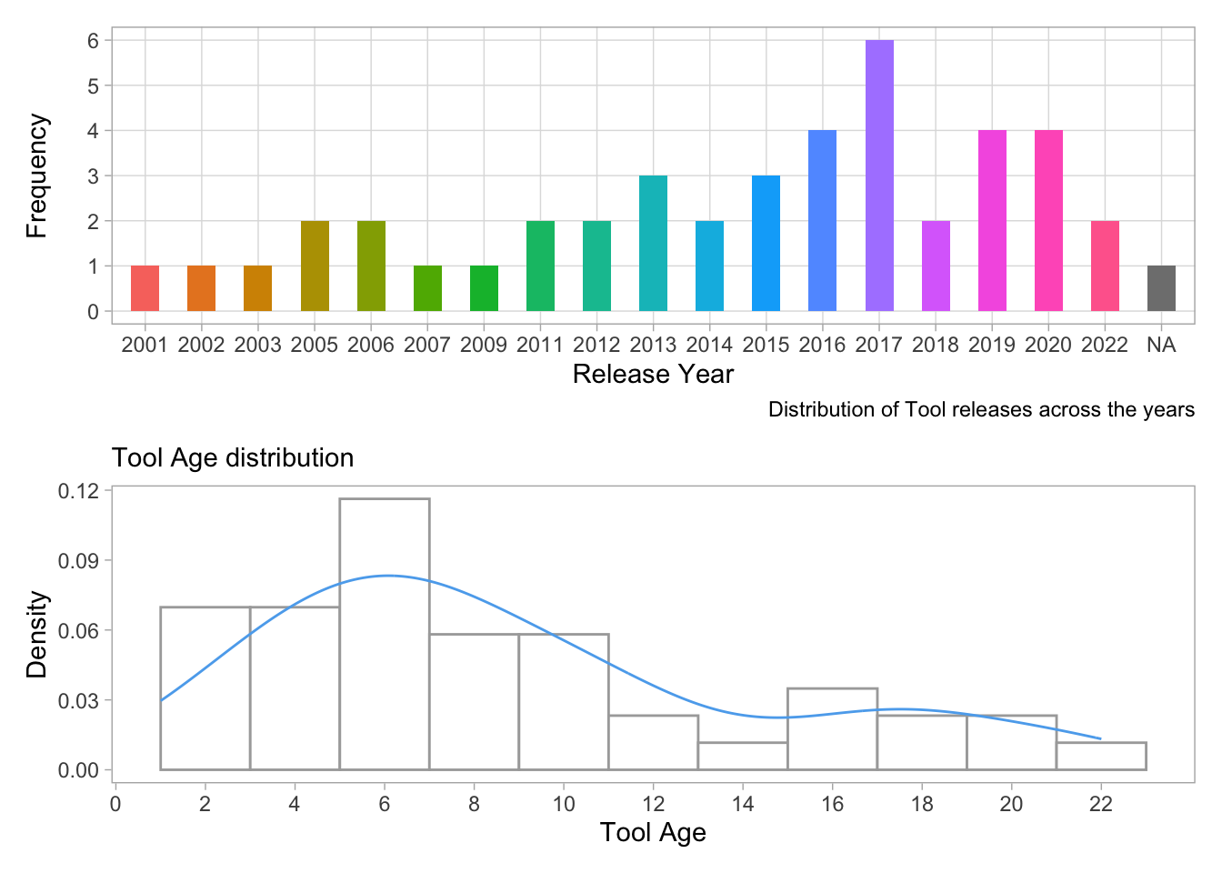

The first plot shows the distribution of tool releases across the years, where the x-axis represents the release year and the y-axis represents the frequency of tool releases. The second plot shows the density distribution of tool age, where the x-axis represents the tool age and the y-axis represents the density of the tool age. The plots suggest that most tools were released in the mid to late 2010s and that the tool age is positively skewed, indicating that most of the tools are relatively new.

7. Time elapsed since last update

p1 <- wdat %>%
  ggplot(aes(x = TimeSinceLastUpdate)) +
  geom_histogram(aes(y = after_stat(density)), fill = "white", col = "darkgray", binwidth = 1) +
  geom_density(col = "steelblue2") +
  scale_x_continuous(breaks = seq(0, 6, by = 1)) +
  labs(x = "Elapsed time (years)", y = "Density", subtitle = "Time elaspsed since last update (those updated in 2022 is considered 0 time elapsed)") +
  theme_light() + 
  theme(panel.grid = element_blank() )

 ## Pattern in update tendencies
p2 <- wdat %>%
  ggplot(aes(x = toolAge, y = TimeSinceLastUpdate)) +
  geom_point(col = "navyblue", shape = 2) + 
  geom_smooth(se = F, col = "steelblue2") + 
  labs(y = "Elapsed time since last update (years)", x = "Tool Age (years)", caption = "No apparent pattern presents itself here") +
  scale_x_continuous(n.breaks = 12) +
  theme_light() + 
  theme(panel.grid = element_blank() )

p1 / p2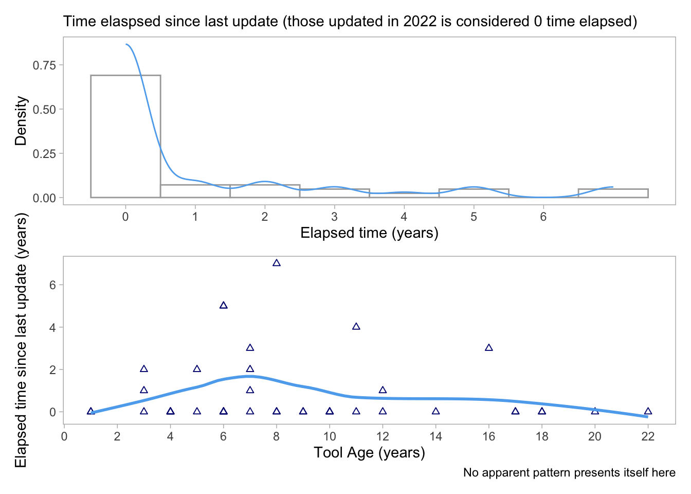

The first plot shows the density distribution of the time elapsed since the last update of the software tools. The x-axis represents the elapsed time in years and the y-axis represents the density of software tools. The plot suggests that a large number of software tools were last updated within the last year, while there is a decrease in the density of software tools that have not been updated for longer periods.
The second plot shows the relationship between the elapsed time since the last update and the age of the software tool. The x-axis represents the age of the software tool, while the y-axis represents the elapsed time since the last update. The plot shows that there is no apparent pattern between the age of the software tool and the elapsed time since the last update.

## Time elapsed since last update - One year vs more
wdat %>% 
  mutate(TimeSinceLastUpdate_bin = if_else(TimeSinceLastUpdate < 2, "<= 1 year", "2+ years")) %>% 
  ggplot(aes(x = TimeSinceLastUpdate_bin, fill = TimeSinceLastUpdate_bin)) +
  geom_bar(position = "dodge", width = .5, show.legend = F) + 
   geom_text(stat = 'count', color = "white",
            aes(label = paste0(after_stat(count))), position = position_dodge(width = .9), vjust = 1.2) +
  labs(x = "Elapsed time category", y = "Frequency", caption = "Time elaspsed since last update (those updated in 2022 is considered 0 time elapsed)") +
  scale_y_continuous(n.breaks = 7) + 
  scale_fill_manual(values = c("#CC79A7", "#009E73")) +
  theme_light() +
  theme(panel.grid = element_blank())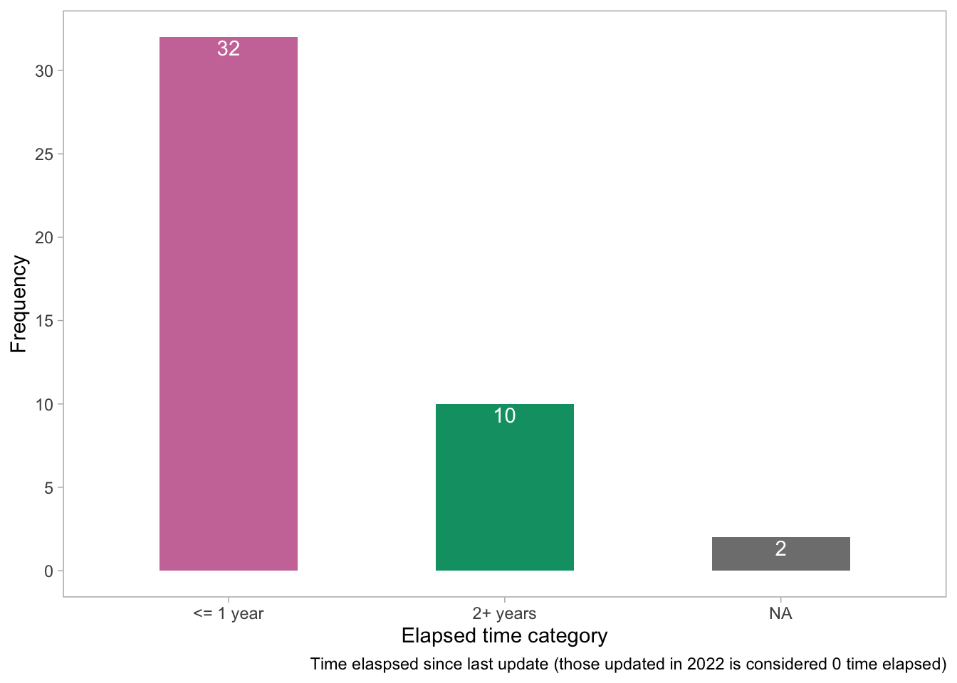

This plot supports the findings from the previous figures and gives a number of those who were updated more than a year ago.

## Time elapsed since last update - One year vs more || Stratified by tool type
wdat %>% 
  mutate(TimeSinceLastUpdate_bin = if_else(TimeSinceLastUpdate < 2, "<= 1 year", "2+ years")) %>% 
  ggplot(aes(x = TimeSinceLastUpdate_bin, fill = TimeSinceLastUpdate_bin)) +
  geom_bar(position = "dodge", width = .5, show.legend = F) + 
  geom_text(stat = 'count', color = "white",
            aes(label = paste0(after_stat(count))), position = position_dodge(width = .9), vjust = 1.1) +
  labs(x = "Elapsed time category", y = "Frequency", caption = "Time elaspsed since last update (those updated in 2022 is considered 0 time elapsed)") +
  facet_wrap(~toolType) +
  scale_y_continuous(n.breaks = 7) + 
  scale_fill_manual(values = c("#CC79A7", "#009E73")) +
  theme_light() +
  theme(strip.background =element_rect(fill="steelblue4"),
        strip.text = element_text(colour = 'white', size = 11),
        panel.grid = element_blank())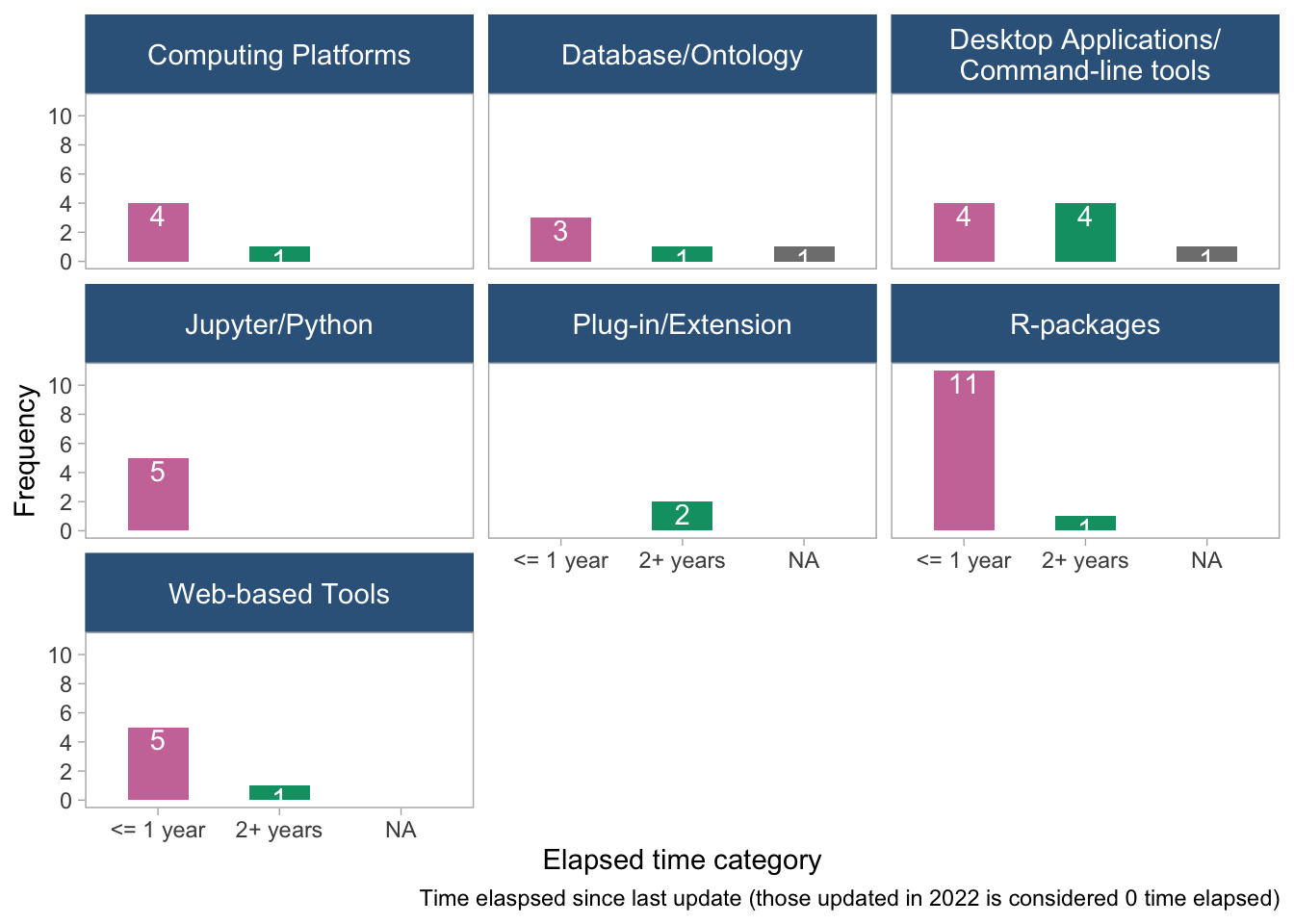

## by data type
## Time elapsed since last update - One year vs more || Stratified
wdat %>% 
  mutate(TimeSinceLastUpdate_bin = if_else(TimeSinceLastUpdate < 2, "<= 1 year", "2+ years")) %>% 
  ggplot(aes(x = TimeSinceLastUpdate_bin, fill = TimeSinceLastUpdate_bin)) +
  geom_bar(position = "dodge", width = .5, show.legend = F) + 
  geom_text(stat = 'count', color = "white",
            aes(label = paste0(after_stat(count))), position = position_dodge(width = .9), vjust = 1.1) +
  labs(x = "Elapsed time category", y = "Frequency", caption = "Time elaspsed since last update (those updated in 2022 is considered 0 time elapsed)") +
  facet_wrap(~dataType) +
  scale_y_continuous(n.breaks = 7) + 
  scale_fill_manual(values = c("#CC79A7", "#009E73")) +
  theme_light() +
  theme(strip.background =element_rect(fill="steelblue4"),
        strip.text = element_text(colour = 'white', size = 11),
        panel.grid = element_blank())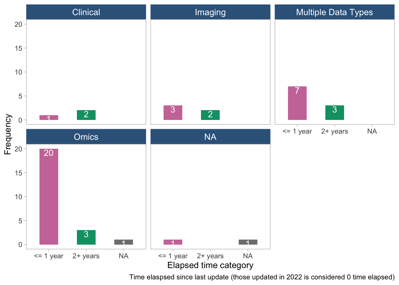

The plots suggest that there is no clear pattern between time elapsed since the last update and tool age or tool/data type. There are a few tools that have been updated more recently, but they appear to be scattered across different tool and data types.

8. Extensive contact/feedback

wdat %>%
  ggplot(aes(y = fct_infreq(extensiveContact), fill = extensiveContact)) +
  geom_bar(position = "dodge", width = .5, show.legend = F) + 
  geom_text(stat = 'count', color = "white",
            aes(label = paste0(after_stat(round(100*count/sum(count),1)), "%")), position = position_dodge(width = .9), hjust = 1.2) +
  labs(x = "Extensive contact/feedback", y = "Frequency", caption = "Distribution of Extensive contact/feedback") +
  scale_x_continuous(n.breaks = 13) + 
  scale_fill_manual(values = c("#CC79A7", "grey50", "#009E73")) +
  theme_light()  +
  theme(panel.grid = element_blank())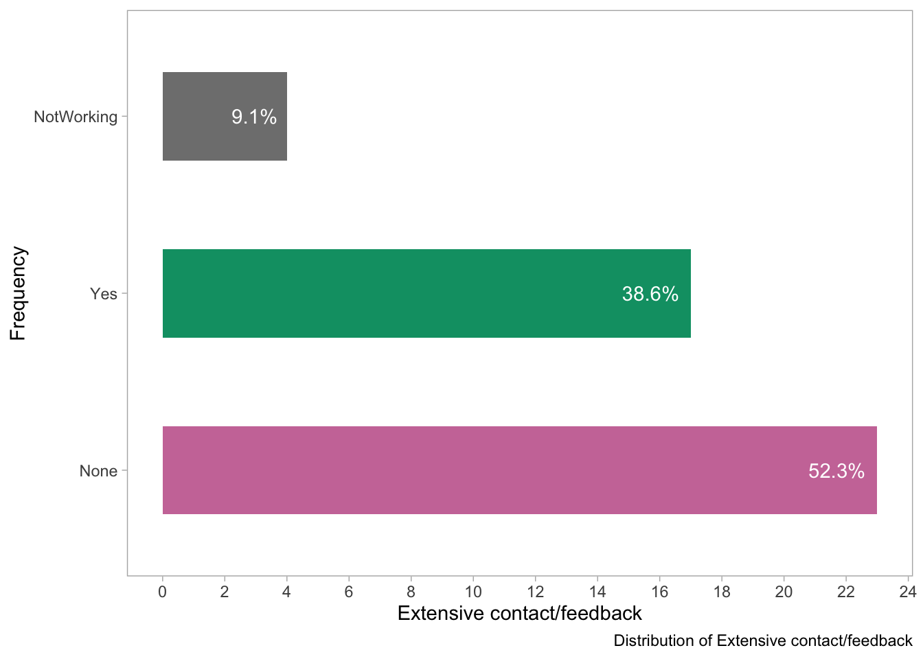

This visualization shows the distribution of responses to the question about whether the tools had extensive contact or feedback methods available with the developers of the tools. It seems that most tools (52.3%) reportedly had very little or no contact or feedback methods. Around one-third (38.6%) reported having extensive contact/feedback methods, 10% of the tools had contact methods that were no longer working/maintained.

## stratified by tool type
wdat %>%
  ggplot(aes(y = fct_infreq(extensiveContact), fill = extensiveContact)) +
  geom_bar(position = "dodge", width = .5, show.legend = F) + 
  geom_text(stat = 'count', color = "white",
            aes(label = paste0(after_stat(count))), position = position_dodge(width = .9), hjust = 1.2) +
  facet_wrap(~toolType) + 
  labs(x = "Extensive contact/feedback", y = "Frequency", caption = "Distribution of Extensive contact/feedback") +
  scale_fill_manual(values = c("#CC79A7", "grey50", "#009E73")) +
  theme_light() +
  theme(strip.background =element_rect(fill="steelblue4"),
        strip.text = element_text(colour = 'white', size = 11),
        panel.grid = element_blank())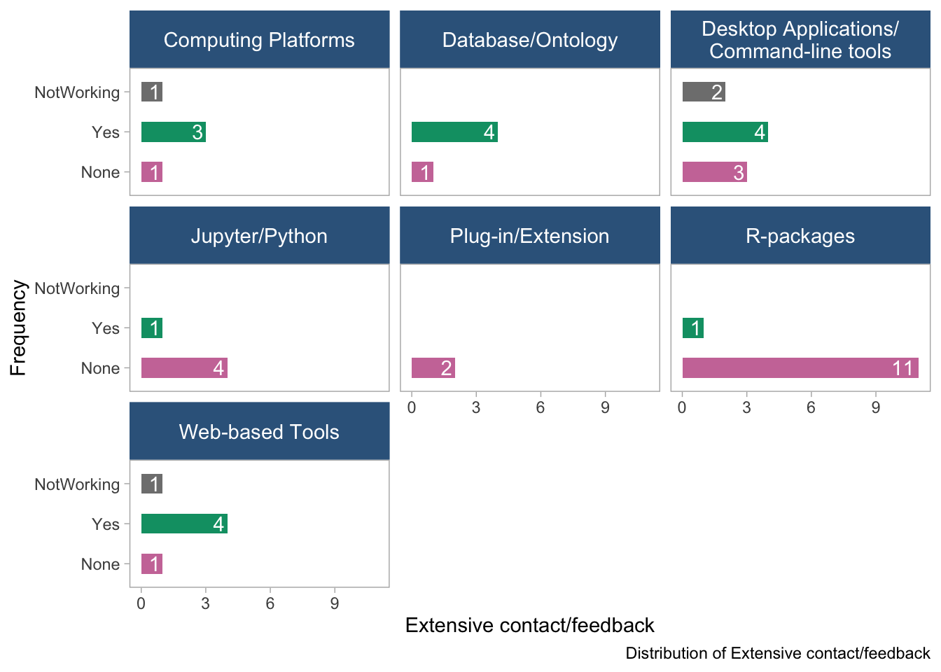

# stratified by data type
wdat %>%
  ggplot(aes(y = fct_infreq(extensiveContact), fill = extensiveContact)) +
  geom_bar(position = "dodge", width = .5, show.legend = F) + 
  geom_text(stat = 'count', color = "white",
            aes(label = paste0(after_stat(count))), position = position_dodge(width = .9), hjust = 1.2) +
  facet_wrap(~dataType) + 
  labs(x = "Extensive contact/feedback", y = "Frequency", caption = "Distribution of Extensive contact/feedback") +
  scale_fill_manual(values = c("#CC79A7", "grey50", "#009E73")) +
  theme_light() +
  theme(strip.background = element_rect(fill="steelblue4"),
        strip.text = element_text(colour = 'white', size = 11),
        panel.grid = element_blank())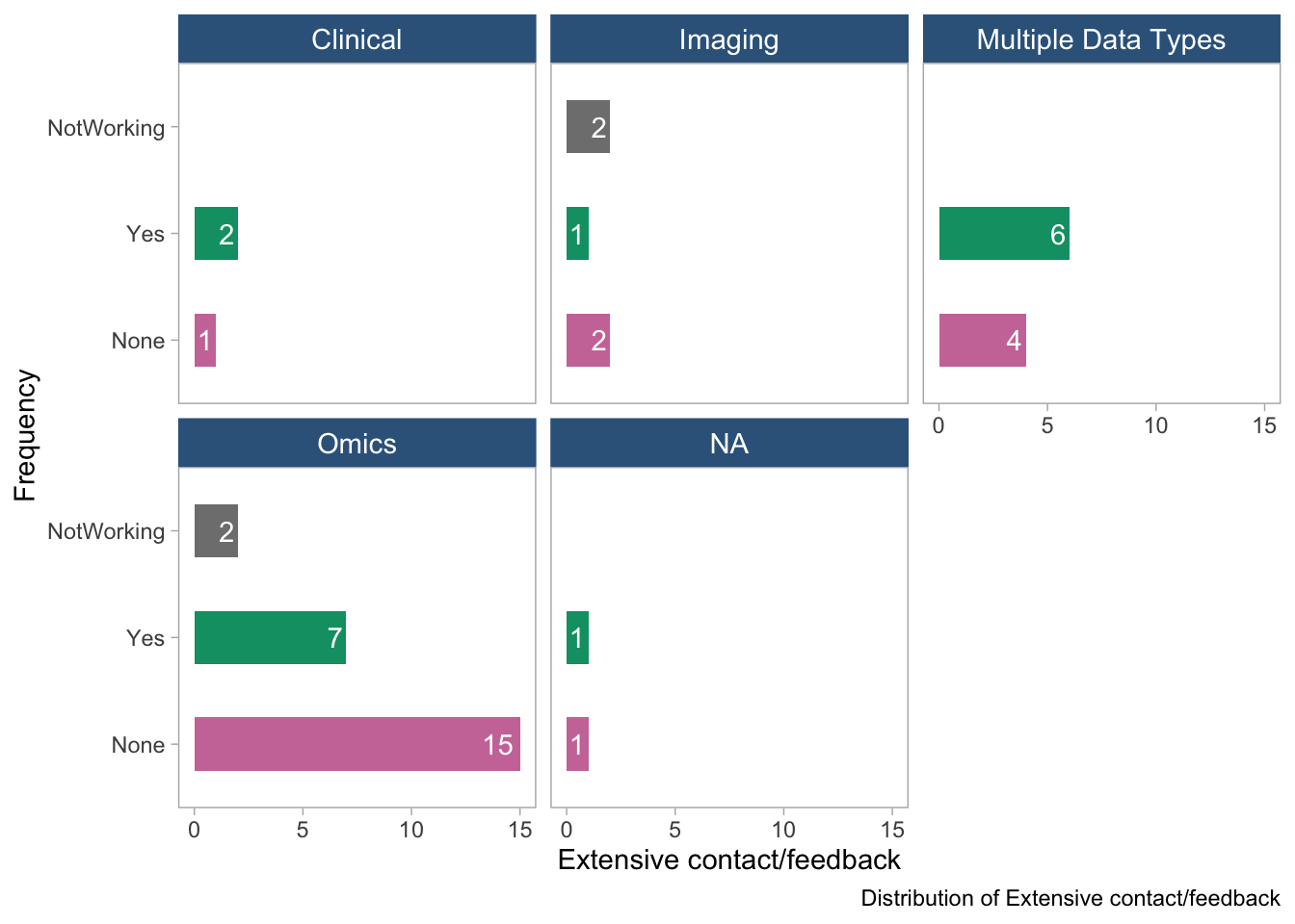

These plots show the distribution of the “extensive contact/feedback” variable in the dataset, stratified by tool type and data type. No clear-cut patterns emerge.

8.2 Checking whether Extensive contact/feedback distributions differ across time categories

wdat %>% filter(!is.na(releaseYear)) %>% 
  mutate(relYear.cut = cut_interval(releaseYear, 4)) %>% 
  ggplot(aes(fill = fct_infreq(extensiveContact), x = relYear.cut)) +
  geom_bar(position = "dodge", width = .5) + 
  # geom_text(stat = 'count', 
  #           aes(label = paste0(after_stat(round(100*count/sum(count),1)), "%")), position = position_dodge(width = .9), hjust = -0.2) +
  labs(x = "Release Year", y = "Frequency", fill = "Extensive contact/feedback") +
  scale_y_continuous(n.breaks = 13) + 
  scale_fill_manual(values = c("#CC79A7", "#009E73", "grey50")) +
  theme_light() +
  theme(panel.grid = element_blank())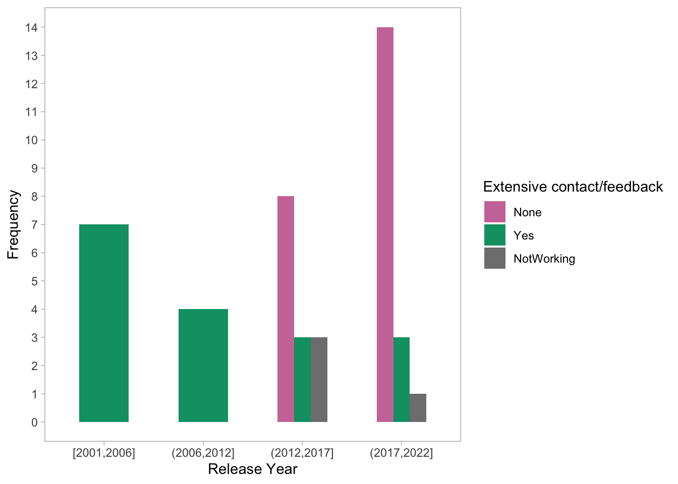

The plot shows the distribution of Extensive contact/feedback across time categories. It appears that there are more instances of extensive contact/feedback in past years (2001-2012) compared to recent years. However, it is important to note that the dataset has more observations for recent years and the older tools might gave had more time to come up with the contact method infrastructures than the newer tools.

## by software metrics
wdat %>% 
  filter(!is.na(releaseYear)) %>% 
  mutate(relYear.cut = cut_interval(releaseYear, 4)) %>% 
  ggplot(aes(fill = fct_infreq(extensiveContact), x = relYear.cut)) +
  geom_bar(position = "dodge", width = .5) + 
  facet_wrap(~simple_health_metrics, nrow = 1) +
  labs(x = "Release Year", y = "Frequency", fill = "Extensive contact/feedback") +
  # scale_y_continuous(n.breaks = 13) + 
  scale_fill_manual(values = c("#CC79A7", "#009E73", "grey50")) +
  theme_light() +
  theme(strip.background =element_rect(fill="steelblue4"),
        strip.text = element_text(colour = 'white', size = 11),
        legend.position = "top", 
        panel.grid = element_blank() ) + 
  coord_flip()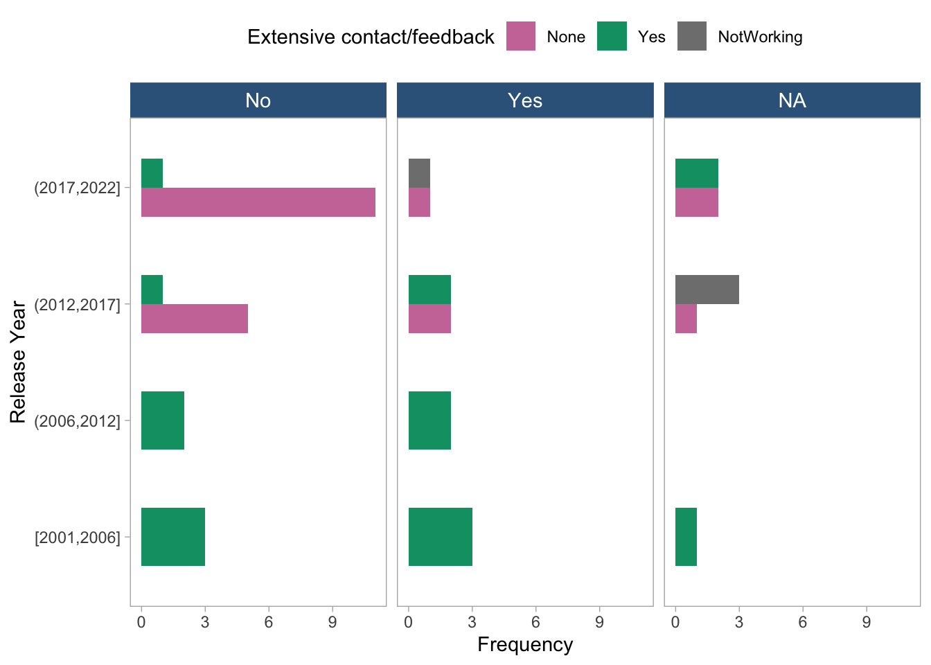

The plot shows the distribution of extensive contact/feedback stratified by release year and simple health metrics. Each panel represents a simple health metric, and the x-axis shows the release year grouped into four-year intervals. The fill color indicates the level of extensive contact/feedback. It seems that the distribution of extensive contact/feedback is relatively consistent across the release years and simple health metrics, with no clear pattern or trend observed.

# Stratified by toolType
wdat %>% filter(!is.na(releaseYear)) %>% 
  mutate(relYear.cut = cut_interval(releaseYear, 4)) %>% 
  ggplot(aes(fill = fct_infreq(extensiveContact), x = relYear.cut)) +
  geom_bar(position = "dodge", width = .5) + 
  facet_wrap(~toolType, nrow = 3) +
  labs(x = "Release Year", y = "Frequency", fill = "Extensive contact/feedback") +
  #scale_y_continuous(n.breaks = 13) + 
  scale_fill_manual(values = c("#CC79A7", "#009E73", "grey50")) +
  theme_light() +
  theme(strip.background =element_rect(fill="steelblue4"),
        strip.text = element_text(colour = 'white', size = 11),
        panel.grid = element_blank(),
        legend.position = "top") + 
  coord_flip()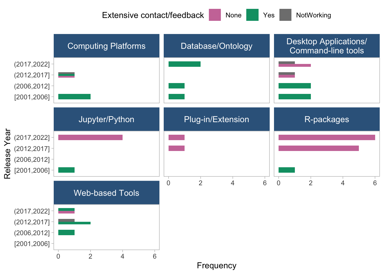

# Stratified by dataType
wdat %>% filter(!is.na(releaseYear)) %>% 
  mutate(relYear.cut = cut_interval(releaseYear, 4)) %>% 
  ggplot(aes(fill = fct_infreq(extensiveContact), x = relYear.cut)) +
  geom_bar(position = "dodge", width = .5) + 
  facet_wrap(~dataType) +
  labs(x = "Release Year", y = "Frequency", fill = "Extensive contact/feedback") +
  #scale_y_continuous(n.breaks = 13) + 
  scale_fill_manual(values = c("#CC79A7", "#009E73", "grey50")) +
  theme_light() +
  theme(strip.background =element_rect(fill="steelblue4"),
        strip.text = element_text(colour = 'white', size = 11),
        panel.grid = element_blank(),
        legend.position = "top") + 
  coord_flip()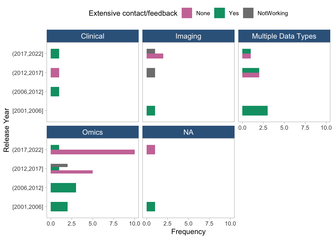

These two plots show the frequency of extensive contact/feedback distribution across release years, stratified by toolType and dataType, respectively. Databases and Web-based tools show extensive contact methods available across the whole period. The patterns are not as clear cut when stratifying by data type.

Part II: Software infrastructure and citation analyses

SoftwareKG-PMC is a database of text-mined software mentions published by Schindler et al 2022(Krüger and Schindler 2020). In principle, this resource enables direct identification and analysis of the usage of ITCR tools in published literature present on PubMedCentral Open Access Subset as of January 2021. We queried the database instance from R using code adapted from the SofwareKG-PMC-Analysis code notebook. The SPARQL library version 1.16 was installed manually from the CRAN archive as the package is no longer maintained. We constructed a query function which returns all articles which mention a given keyword (i.e., software name) in a particular mention category (allusion, usage, creation, or deposition). This yielded 73095 article-level mentions of any type, corresponding to 60970 unique articles for 36 ITCR tool name keywords. 8 tools were not identified, possibly due to recency of release, complexity of the tool name, or gaps in the accuracy or completeness of SoftwareKG and/or PubMedCentral. We further note that results are contaminated to a varying degree by software name homonyms. This type of collision is a chief limitation of SoftwareKG-PMC, especially for tools with simple or generic names. The query was performed in a case-insensitive manner due to the tendency for authors to adjust the capitalization of software names, such as JBrowse vs Jbrowse. SoftwareKG-PMC does not reliably aggregate these variations.

Software mentions was categorized into four types: allusion, usage, creation, and deposition. We distinguish the aforementioned classifications of mention types as follows:

Allusion: This type of mention simply refers to the name of the software and does not require any indication of its usage. Allusions are used to state a fact about the software or to compare multiple software options for a problem. These are similar to the typical scholarly citations used to refer to related work.

Usage: A usage type mention occurs when software is used in an investigation and makes a contribution to the study. This type of mention allows for conclusions about the study’s origins and can be used to develop impact metrics.

Creation: It is a creation mention when a new software is introduced in a publication. This type of mention can be used to provide scholarly credit to the software’s authors, as well as map new creations and track down original software publications.

Deposition: The publication of new software is regarded as a deposition mention. By including information about the publication, such as a license or URL, this expands on the creation type mention. When describing availability and licensing information for software, cross-references are used to annotate indirect statements about the software.

Our analyses fully excluded the creation type mentions. We focused on the usage type mentions as this metric facilitates the evaluation of impact of the software tools better than the other mention types.

Total mentions: total number of articles that either had an allusion or usage or deposition regarding a specific software tool.

Data loading and check

## Load data file: regdat: The SoftwareKG data merged with tool analysis data
regdat <- read_csv(file = "softwareKG_anonymized.csv") %>% 
  mutate(simple_health_metrics = case_when(
    str_detect(health_metrics, "no|No|unknown status|no badge|Not for core software|CI but not badge|\\?") ~ "No",
    str_detect(health_metrics, "Yes|yes|Test badges|CI and coverage badges|bioconductor only| with badge")~ "Yes",
    TRUE ~ health_metrics))

regdat %<>% 
  mutate(dataType = case_when(
    str_detect(`type of data`, "DNA methylation and gene expression|Gene sets|genomics|methylation|microbiome sequence analysis|mostly proteomics|multi-omics|mutation analysis|phenotypic associations|protein-protein interaction networks|genomic, phenotypic") ~ "Omics",
    str_detect(`type of data`, "cancer models|clinical study metadata harmonization|clinical text") ~ "Clinical",
    str_detect(`type of data`, "digital pathology slides|Imaging|PET/CT image analysis|image analysis") ~ "Imaging",
    str_detect(`type of data`, "multi-omics|mixed|genomic|Analysis of Variants") ~ "Multiple Data Types",
    TRUE ~ `type of data`))

## Recode type of tool into simple classification

regdat %<>% rename(toolType = `class/type`) %>% 
  mutate(
    toolType = case_when(
      str_detect(toolType, "Suite") ~ "Suite",
      str_detect(toolType, "Platform") ~ "Computing Platforms",
      str_detect(toolType, "Command-line tool/Other scripts|Desktop Application") ~ "Desktop Applications/\nCommand-line tools",
      str_detect(toolType, "Web") ~ "Web-based Tools",
      str_detect(toolType, "Jupyter|Python") ~ "Jupyter/Python",
      str_detect(toolType, "R") ~ "R-packages",
      TRUE ~ toolType
    )
  )

1. Frequency of different mode of mentions

Note that the last four columns (Allusion, Creation, Deposition, Usage) Need Not sum to the total article mentions as one or more of these different type of mentions may have occurred for a speicific tool in each article.

regdat %>% select(`Anonymous ID` = anonID, totalMentions, Allusion, Deposition, Usage) %>% 
  arrange(desc(totalMentions)) %>% 
  DT::datatable(caption = htmltools::tags$caption("Frequency of different mode of mentions", style = "color:blue"),
                options = list(columnDefs = list(list(className = 'dt-center', targets = "_all"))))

2. Possible association between twitter presence and log(totalMentions)

Note that we are using log-scaled data since the data is count-type and there is considerable variation in it.

## Marginal dist
p1 <- regdat %>% 
  ggplot(aes(x = socialMedia, fill = fct_infreq(socialMedia))) + 
  geom_bar(position = "dodge", width = .5, show.legend = F) + 
  geom_text(stat = 'count', 
            aes(label = paste0(after_stat(round(100*count/sum(count),1)), "%")), 
            position = position_dodge(width = .9), vjust = 2, col = "white") +
  labs(x = "Twitter Presence", y = "Frequency", subtitle = "Distribution of Twitter Presence") +
  scale_y_continuous(n.breaks = 7) + 
  scale_fill_manual(values = c("#CC79A7", "#009E73")) +
  theme_light() +
  theme(panel.grid = element_blank())

p2 <- regdat %>% 
  ggplot(aes(x = socialMedia, y = log(totalMentions))) +
  geom_boxplot(aes(fill = socialMedia),  width = 0.5, show.legend = F) +
  scale_y_continuous(n.breaks = 6) + 
  scale_fill_manual(values = c("#CC79A7", "#009E73")) +
  labs(x = "Twitter Presence", y = "log( total # of total mentions)", 
       subtitle = "Distribution of # of total mentions (log scale)") +
  theme_light() +
  theme(panel.grid = element_blank())

p1 + p2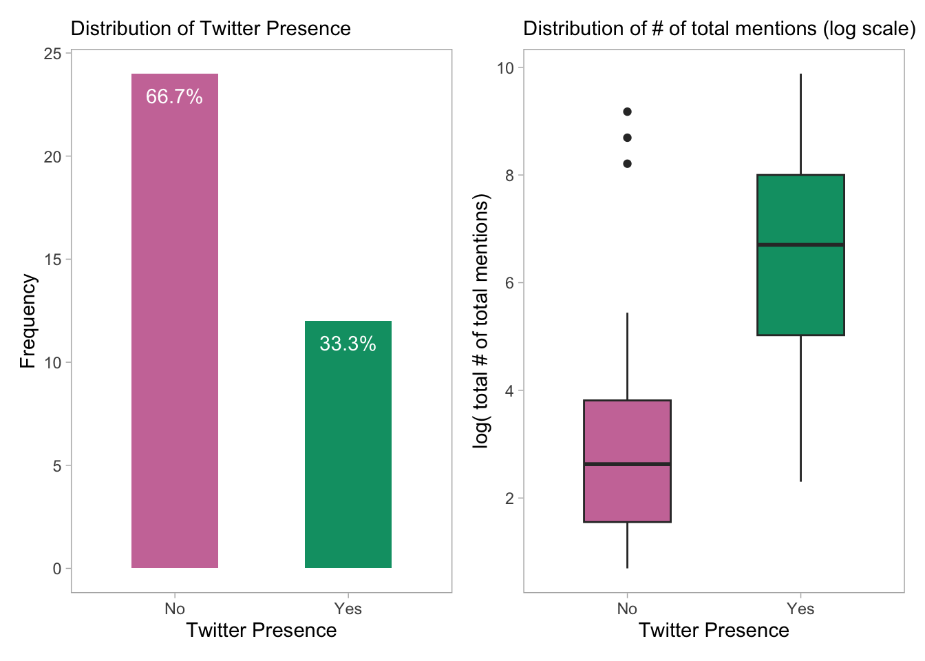

The plots show the distribution of Twitter presence among the software tools included in the data and the distribution of the total number of mentions on Twitter for each tool. The left panel plot shows that the majority of tools do not have a Twitter presence, while a smaller number have a presence on Twitter. The second plot shows that the number of mentions for each tool on Twitter varies widely, but those with Twitter have a higher median citation/mention count. The distribution of mentions is shown on a log scale.

## Allusions
p21 <- regdat %>% filter(!is.na(Allusion)) %>% 
  ggplot(aes(x = socialMedia, y = log(Allusion))) +
  geom_boxplot(aes(fill = socialMedia),  width = 0.5, show.legend = F) +
  scale_y_continuous(n.breaks = 6) + 
  scale_fill_manual(values = c("#CC79A7", "#009E73")) +
  labs(x = "Twitter Presence", y = "log(Allusion)", subtitle = "Distribution of # of Allusion (log scale)") +
  theme_light() + coord_flip() +
  theme(panel.grid = element_blank())

## Deposition
p23 <- regdat %>% filter(!is.na(Deposition)) %>% 
  ggplot(aes(x = socialMedia, y = log(Deposition))) +
  geom_boxplot(aes(fill = socialMedia),  width = 0.5, show.legend = F) +
  scale_y_continuous(n.breaks = 6) + 
  scale_fill_manual(values = c("#CC79A7", "#009E73")) +
  labs(x = "Twitter Presence", y = "log(Deposition)", 
       subtitle = "Distribution of # of Deposition (log scale)") +
  theme_light() + coord_flip() +
  theme(panel.grid = element_blank())

## Usage
p24 <- regdat %>% filter(!is.na(Usage)) %>% 
  ggplot(aes(x = socialMedia, y = log(Usage))) +
  geom_boxplot(aes(fill = socialMedia),  width = 0.5, show.legend = F) +
  scale_y_continuous(n.breaks = 6) + 
  scale_fill_manual(values = c("#CC79A7", "#009E73")) +
  labs(x = "Twitter Presence", y = "log(Usage)", subtitle = "Distribution of # of Usage (log scale)") +
  theme_light() + coord_flip() +
  theme(panel.grid = element_blank())

(p24) / (p21 + p23)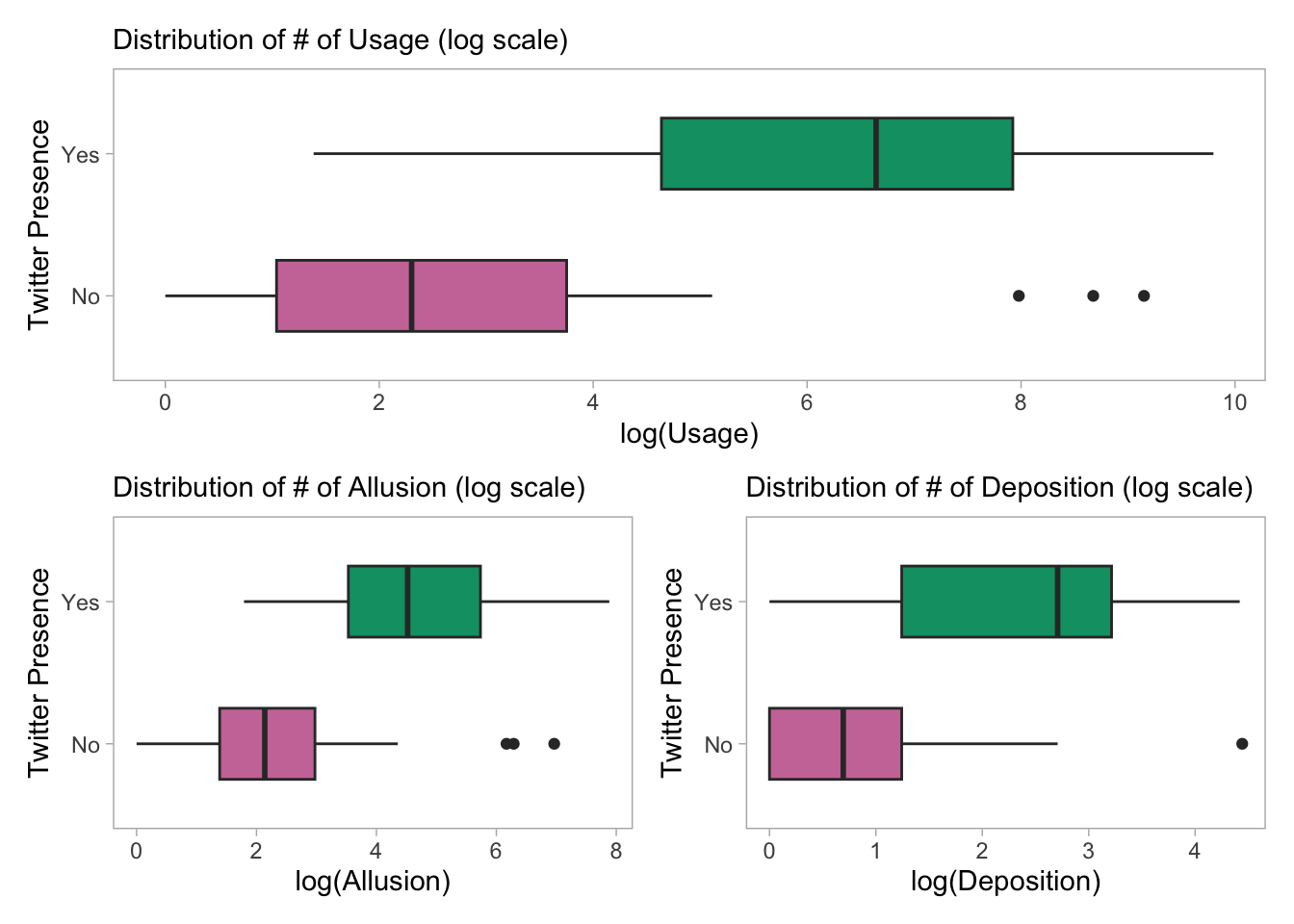

It appears that the distribution of log-frequency (and hence the frequency) for each of Usage, Allusion and Deposition differ considerably. But the distribution of Usage for Twitter user and non-user tools is considerably constrasting.
However, mention is a function of time as well. So we need to check whether adjusting age of tool affects this crude association.

p3 <- regdat %>% 
  ggplot(aes(x = releaseYear, y = log(totalMentions), col = socialMedia)) + 
  geom_point(aes(shape = socialMedia)) + 
  geom_smooth(method = "lm", se = F) +
  scale_color_manual(values = c("#CC79A7", "#009E73")) +
  labs(x = "Release Year", y = "log(total Mentions)", col = "Twitter \npresence", shape = "Twitter \npresence",
       subtitle = "Scatterplot of log-totalMentions vs Release Year") +
  theme_light() 

p3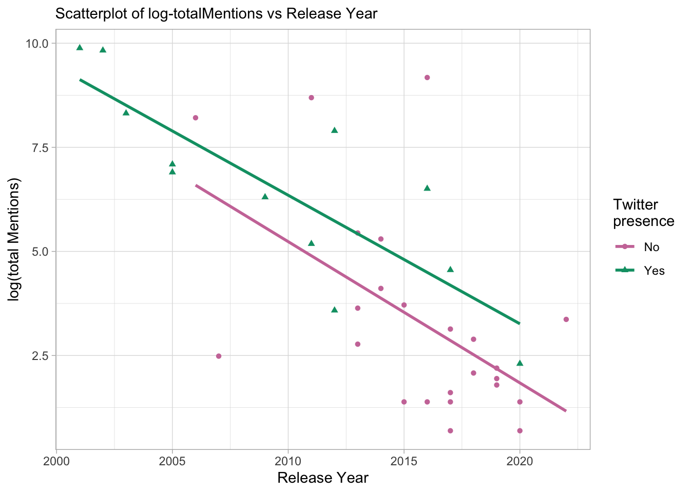

The plot shows a generally positive association between log-transformed total mentions and release year (or negative association between tool/software age and total mentions), which suggests that the age of a tool may have an impact on the number of mentions it receives. The presence of Twitter seems to have a relatively weak association with the number of mentions, but tools with a Twitter presence appear to be generally more recent than those without.

2.2 Exploratory regression models

lm(log(totalMentions) ~ Twitter, data = regdat %>% rename(Twitter = socialMedia)) %>% broom::tidy() %>% 
  mutate(across(.cols = where(is.numeric), .fns = ~round(.x, digits = 4))) %>% 
  DT::datatable()

lm(log(totalMentions) ~ Twitter + toolAge, data = regdat %>% rename(Twitter = socialMedia)) %>% broom::tidy() %>% 
  mutate(across(.cols = where(is.numeric), .fns = ~round(.x, digits = 5))) %>% 
  DT::datatable()

The first model includes only Twitter presence as a predictor variable, while the second model includes both Twitter presence and tool age as predictor variables. The first model shows that tools with a Twitter presence have significantly higher log of total mentions than those without a Twitter presence (estimate = 3.2, p-value < 0.001). The second model shows that the association between Twitter presence and log of total mentions no longer remains significant when controlling for tool age, which has a significant positive association with log of total mentions (estimate = 0.322, p-value < 0.001).
So adjusting for Tool age (a translation of release Year) shows that Twitter presence is not significant. The variability is too high to conclude anything statistically. It seems that Tool age is a very strong predictor of the log(TotalMentions), and makes the other variables insignificant.

3. Stratification by: How to cite instructions available (with BioConductor)

Instruction on How to cite: The binary variable “Instruction on How to cite” specifies whether each tool provides instructions on how to properly cite it in a research publication or other work. These instructions typically include information such as the author(s) names, version number, publication date, and website or repository where the tool can be found. Tools that do not provide such instructions can make it difficult for researchers to correctly cite the tool, potentially leading to incomplete or inaccurate acknowledgements of its use in research.

## Marginal dist
p4 <- regdat %>% 
  ggplot(aes(x = citeHow, fill = fct_infreq(citeHow))) + 
  geom_bar(position = "dodge", width = .5, show.legend = F) + 
  geom_text(stat = 'count', 
            aes(label = paste0(after_stat(round(100*count/sum(count),1)), "%")), 
            position = position_dodge(width = .9), vjust = 2, col = "white") +
  labs(x = "Instruction for citation", y = "Frequency", subtitle = "Distribution of Presence of Citation instructions") +
  scale_y_continuous(n.breaks = 7) + 
  scale_fill_manual(values = c( "#009E73", "#CC79A7")) +
  theme_light() +
  theme(panel.grid = element_blank())

p5 <- regdat %>% 
  ggplot(aes(x = citeHow, y = log(totalMentions))) +
  geom_boxplot(aes(fill = citeHow),  width = 0.5, show.legend = F) +
  scale_y_continuous(n.breaks = 6) + 
  scale_fill_manual(values = c("#CC79A7", "#009E73")) +
  labs(x = "Instruction for citation", y = "log( total # of mentions)", 
       subtitle = "Distribution of # of mentions (log scale)") +
  theme_light() +
  theme(panel.grid = element_blank())

p4 + p5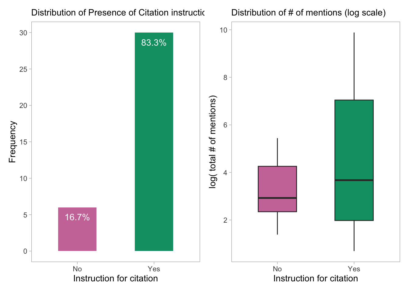

The plot shows the distribution of the number of mentions (log scale) for each type of citation instruction. There does not seem to much difference in the distribution of log-citations across the two categories but the tools with citation instructions have a higher variability of citation/mention counts.

regdat %>% 
  ggplot(aes(x = citeHow, y = log(totalMentions))) +
  geom_boxplot(aes(fill = socialMedia),  width = 0.5, ) +
  scale_y_continuous(n.breaks = 6) + 
  #facet_wrap(~`class/type`) +
  scale_fill_manual(values = c("#CC79A7", "#009E73")) +
  labs(x = "Instructions on how to cite?", y = "log( total # of mentions)", 
       fill = "Twitter \npresence",
       subtitle = "Distribution of # of mentions (log scale)") +
  theme_light() +
  theme(strip.background = element_rect(fill="steelblue4"),
        strip.text = element_text(colour = 'white'), 
        panel.grid = element_blank())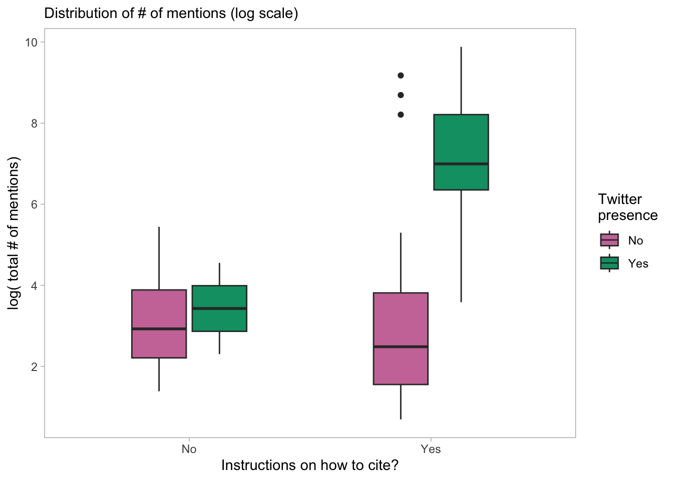

lm(log(totalMentions) ~ Twitter + citeHow + Twitter:citeHow, data = regdat %>% rename(Twitter = socialMedia)) %>% 
  broom::tidy() %>% 
  mutate(across(.cols = where(is.numeric), .fns = ~round(.x, digits = 5))) %>% 
  DT::datatable()

The interaction term is not significant, suggesting that the effect of Twitter presence on log(totalMentions) is not different across different types of citation instruction.

4. Stratification by: How to cite instruction (WITHOUT BioConductor and other-R packages)

## Marginal dist
p41 <- regdat %>% filter(toolType != c("Bioconductor R packages", "other R packages")) %>% 
  ggplot(aes(x = citeHow, fill = fct_infreq(citeHow))) + 
  geom_bar(position = "dodge", width = .5, show.legend = F) + 
  geom_text(stat = 'count', 
            aes(label = paste0(after_stat(round(100*count/sum(count),1)), "%")), 
            position = position_dodge(width = .9), vjust = 1.2, col = "white") +
  labs(x = "Instruction for citation", y = "Frequency", subtitle = "Distribution of Presence of Citation instructions") +
  scale_y_continuous(n.breaks = 7) + 
  scale_fill_manual(values = c("#009E73", "#CC79A7")) +
  theme_light() +
  theme(panel.grid = element_blank())

p51 <- regdat %>% filter(toolType != c("Bioconductor R packages", "other R packages")) %>% 
  ggplot(aes(x = citeHow, y = log(totalMentions))) +
  geom_boxplot(aes(fill = citeHow),  width = 0.5, show.legend = F) +
  scale_y_continuous(n.breaks = 6) + 
  scale_fill_manual(values = c("#CC79A7", "#009E73")) +
  labs(x = "Instruction for citation", y = "log( total # of mentions)", 
       subtitle = "Distribution of # of mentions (log scale)") +
  theme_light() +
  theme(panel.grid = element_blank())


p61 <- regdat %>% filter(toolType != c("Bioconductor R packages", "other R packages")) %>% 
  ggplot(aes(x = citeHow, y = log(totalMentions))) +
  geom_boxplot(aes(fill = socialMedia),  width = 0.5, ) +
  scale_y_continuous(n.breaks = 6) + 
  scale_fill_manual(values = c("#CC79A7", "#009E73")) +
  labs(x = "Instructions on how to cite?", y = "log( total # of mentions)", fill = "Twitter \npresence",
       subtitle = "Distribution of # of mentions (log scale)") +
  theme_light() +
  theme(strip.background =element_rect(fill="steelblue4"),
        strip.text = element_text(colour = 'white'), 
        panel.grid = element_blank())

(p41 + p51) /
  p61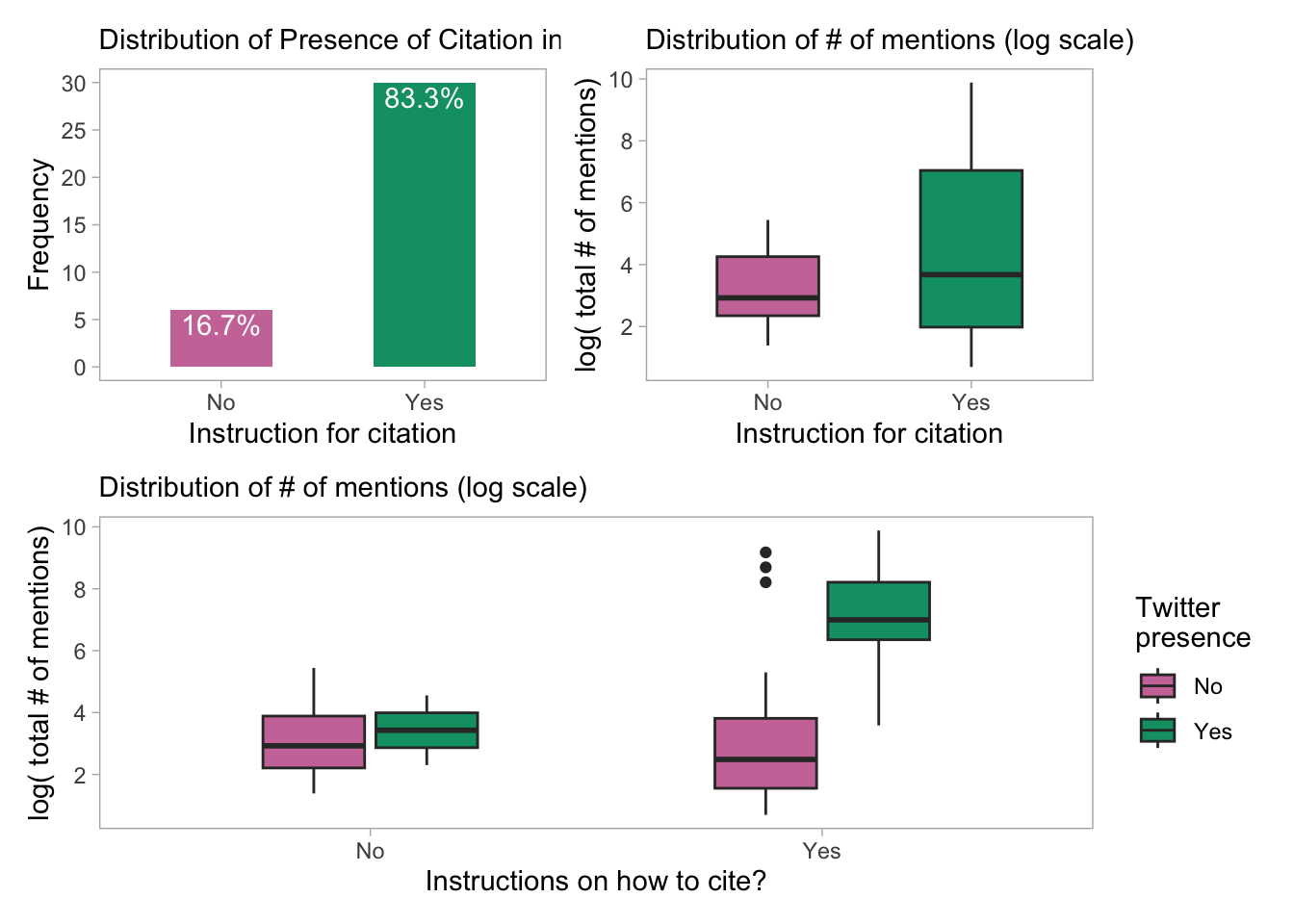

lm(log(totalMentions) ~ Twitter + citeHow + Twitter:citeHow, data = regdat %>% rename(Twitter = socialMedia) %>%  filter(toolType != c("Bioconductor R packages", "other R packages"))) %>% 
  broom::tidy() %>% 
  mutate(across(.cols = where(is.numeric), .fns = ~round(.x, digits = 5))) %>% 
  DT::datatable()

Inclusion or exclusion of R-packages (which have different citation/mention dynamics) does not alter our conclusions.

5. Stratification by: extensiveContact

Extensive Contact: The binary variable “Extensive Contact Methods” indicates whether a tool offers multiple ways for users to contact developers for support or other inquiries, such as email addresses, discussion boards, contact forms, and more. Tools with several contact options may be more user-friendly as they enable researchers to seek support or report issues with the tool more conveniently and effectively. In contrast, tools with inadequate or no contact methods may be less attractive to researchers, as they don’t provide timely help for technical difficulties or other concerns.

regdat %>% mutate(extensiveContact = if_else(extensiveContact == "None", extensiveContact, "Yes")) %>% 
  ggplot(aes(x = extensiveContact, y = log(totalMentions))) +
  geom_boxplot(aes(fill = extensiveContact), width = 0.4, show.legend = F) +
  scale_y_continuous(n.breaks = 6) + 
  #facet_wrap(~`class/type`) +
  scale_fill_manual(values = c("#CC79A7", "#009E73")) +
  labs(x = "Extensive Contact method availability", y = "log( total # of mentions)", 
       subtitle = "Distribution of # of mentions (log scale)") +
  theme_light() +
  theme(strip.background = element_rect(fill="steelblue4"),
        strip.text = element_text(colour = 'white'), 
        panel.grid = element_blank()) + 
  coord_flip()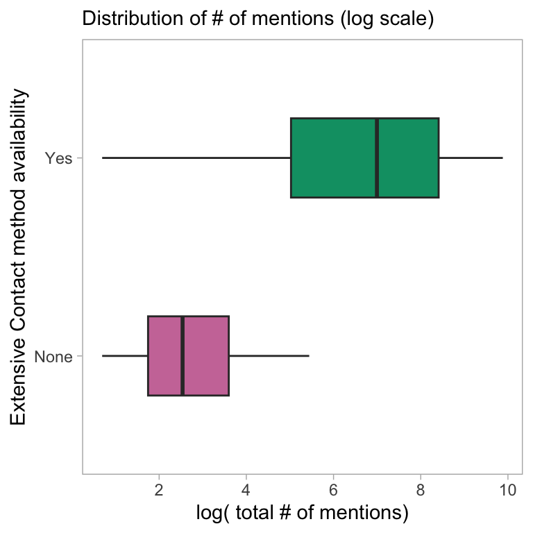

regdat %>% mutate(extensiveContact = if_else(extensiveContact == "None", extensiveContact, "Yes")) %>% 
lm(log(totalMentions) ~ extensiveContact + toolAge, data = .) %>% broom::tidy() %>% 
  mutate(across(.cols = where(is.numeric), .fns = ~round(.x, digits = 5))) %>% 
  DT::datatable()

regdat %>% rename(Twitter = socialMedia) %>% 
  mutate(extensiveContact = if_else(extensiveContact == "None", extensiveContact, "Yes")) %>% 
lm(log(totalMentions) ~ extensiveContact + toolAge + Twitter, data = .) %>% broom::tidy() %>% 
  mutate(across(.cols = where(is.numeric), .fns = ~round(.x, digits = 5))) %>% 
  DT::datatable()

Here the distribution of the log of the total number of mentions is stratified by the availability of an extensive contact method, and two linear models are fit to explore the association of this variable with the outcome variable while adjusting for the tool age and Twitter presence. There seems to be considerable difference in the distribution of mention/citation counts across the tools that differ in the extensive contact methods availability.
Having Extensive contact method available is significant Even After adjusting for Tool age and Twitter presence. Clearly, this is an important feature governing the usage and popularity of the tool.

6. Stratification by: Documentation Depth

Documentation depth: The binary variable “Documentation depth” characterizes the degree of documentation for each tool as either “extensive” or “Webpage/PDF/ReadMe”. The term extensive documentation refers to comprehensive resources such as user guides, training, tutorials, code examples, and FAQs that allow users to better understand the functionality of the tools and interpret their outputs. The “Webpage/PDF/ReadMe” category, on the other hand, designates that the tool offers less information, possibly in the form of a website, PDF, or readme file. This “Webpage/PDF/ReadMe” category can be interpreted as having a lower level of documentation depth, as it typically provides users with a more basic level of information about the tool. This type of documentation may only include a brief description of the tool, its features, and how to install it without going into more detailed instructions or use cases. The “Webpage/PDF/ReadMe” category may be sufficient for users who are already familiar with similar tools or have prior experience in the field, but it may not provide enough guidance for beginners or users who need more detailed instructions to use the tool effectively. Therefore, having a higher level of documentation depth, such as “extensive,”, can be beneficial for both novice and experienced users, as it provides more detailed information, tutorials, and use cases, making it easier for them to learn about the tool and utilize it to its full potential.

## Marginal dist
p_doc1 <- regdat %>%  
  ggplot(aes(x = DocuDepth, fill = fct_infreq(DocuDepth))) + 
  geom_bar(position = "dodge", width = .5, show.legend = F) + 
  geom_text(stat = 'count', 
            aes(label = paste0(after_stat(round(100*count/sum(count),1)), "%")), 
            position = position_dodge(width = .9), vjust = 2, col = "white") +
  labs(x = "Documentation depth", y = "Frequency", subtitle = "Distribution of Documentation \ndepth") +
  scale_y_continuous(n.breaks = 7) + 
  scale_fill_manual(values = c("#009E73", "#CC79A7")) +
  theme_light() +
  theme(panel.grid = element_blank())

p_doc2 <- regdat %>%
  ggplot(aes(x = DocuDepth, y = log(totalMentions), fill = DocuDepth)) +
  geom_boxplot(width = 0.5, show.legend = T) +
  scale_y_continuous(n.breaks = 6) + 
  scale_fill_manual(values = c("#009E73", "#CC79A7")) +
  labs(x = "Documentation depth", y = "log( total # of mentions)", fill = "Documentation depth",
       subtitle = "Distribution of # of total mentions \n(log scale)") +
  theme_light() +
  theme(panel.grid = element_blank())

p_doc1 + p_doc2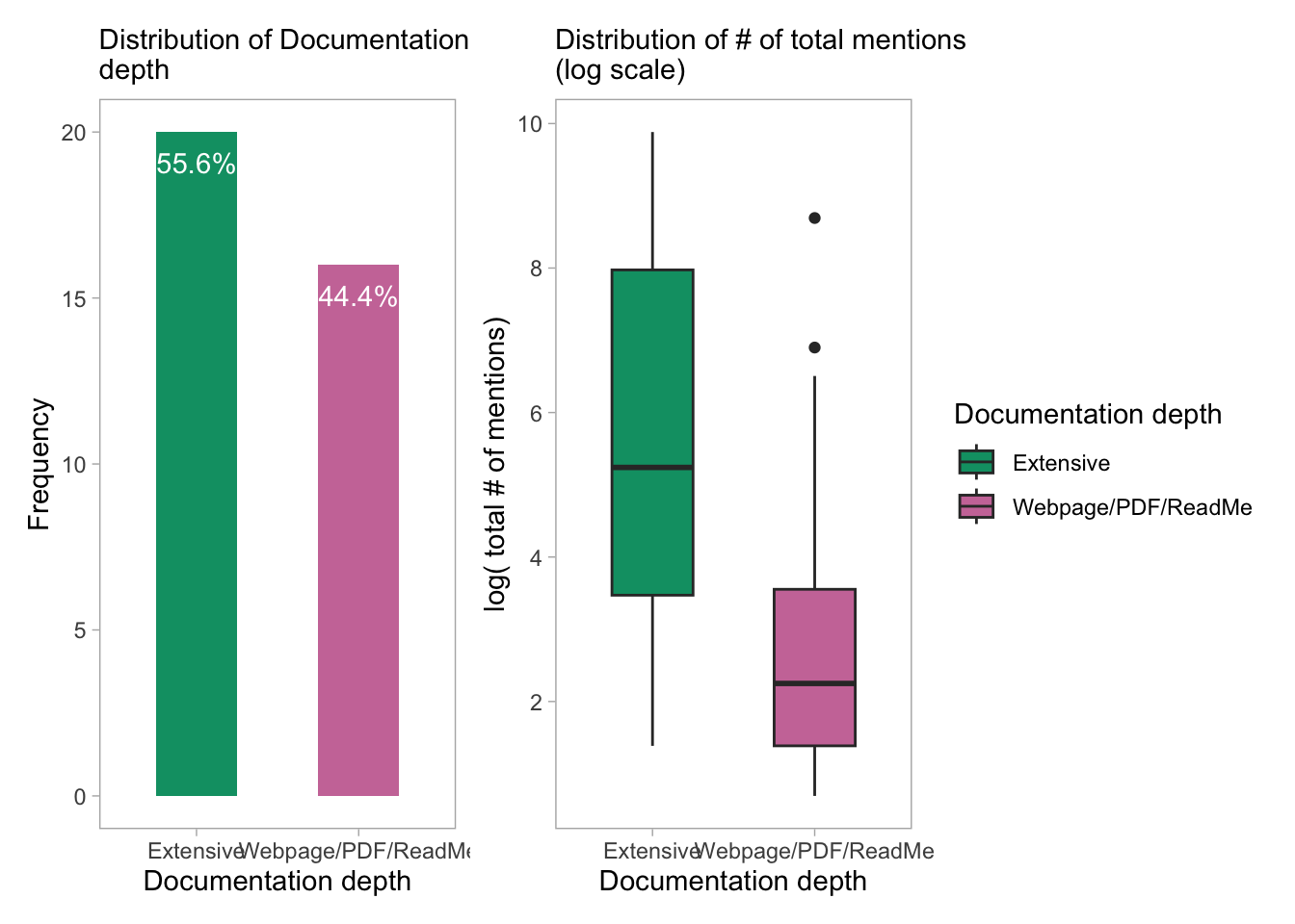

Tools with a “high” level of documentation depth tend to have more mentions compared to those with “low” and “medium” levels. This trend is supported by the boxplot showing the distribution of total mentions for each level of documentation depth.

lm(log(totalMentions) ~ DocuDepth, data = regdat) %>% broom::tidy() %>% 
  mutate(across(.cols = where(is.numeric), .fns = ~round(.x, digits = 5))) %>% 
  DT::datatable()

regdat %>% mutate(extensiveContact = if_else(extensiveContact == "None", extensiveContact, "Yes")) %>% 
lm(log(totalMentions) ~ extensiveContact + DocuDepth + toolAge, data = .) %>% broom::tidy() %>% 
  mutate(across(.cols = where(is.numeric), .fns = ~round(.x, digits = 5))) %>% 
  DT::datatable()

lm(log(totalMentions) ~ DocuDepth + socialMedia + extensiveContact + toolAge, data = regdat) %>% broom::tidy() %>% 
  mutate(across(.cols = where(is.numeric), .fns = ~round(.x, digits = 5))) %>% 
  DT::datatable()

#names(regdat)

7. Trend using “total Usage”

# Twitter
d1 <- regdat %>% 
  ggplot(aes(x = releaseYear, y = log(Usage), col = socialMedia)) + 
  geom_point(aes(shape = socialMedia)) + 
  geom_smooth(method = "lm", se = T, alpha = 0.2) +
  labs(x = "Release Year", y = "log(total Usage)", col = "Twitter \nPresence", shape = "Twitter \nPresence", 
       title = "Twitter Presence") +
  scale_color_manual(values = c("#CC79A7", "#009E73")) +
  theme_light() + 
  coord_equal() + 
  theme(legend.position = "bottom",
        aspect.ratio = .6)

## DocuDepth
d2 <- regdat %>%
  mutate(DocuDepth = fct_recode(DocuDepth, "Webpage/PDF/\nReadMe" = "Webpage/PDF/ReadMe")) %>% 
  ggplot(aes(x = releaseYear, y = log(Usage), col = DocuDepth)) + 
  geom_point(aes(shape = DocuDepth)) + 
  geom_smooth(method = "lm", se = T, alpha = 0.2) +
  labs(x = "Release Year", y = "log(total Usage)", col = "Documentation \nDepth", shape = "Documentation \nDepth", title = "Documentation Depth") +
  scale_color_manual(values = c("#009E73", "#CC79A7")) +
  theme_light() + 
  coord_equal() + 
  theme(legend.position = "bottom",
        aspect.ratio = .6)

# extensiveContact
d3 <- regdat %>% mutate(extensiveContact = if_else(extensiveContact == "None", "Little or no \ncontact methods", "Extensive \nmethods")) %>% 
  ggplot(aes(x = releaseYear, y = log(Usage), col = extensiveContact)) + 
  geom_point(aes(shape = extensiveContact)) + 
  geom_smooth(method = "lm", se = T, alpha = 0.2) +
  labs(x = "Release Year", y = "log(total Usage)", col = "Contact \nMethods", shape = "Contact \nMethods", 
       title = "Contact Methods") +
  scale_color_manual(values = c("#009E73", "#CC79A7")) +
  theme_light() + 
  coord_equal() + 
  theme(legend.position = "bottom",
        aspect.ratio = .6)

# CiteHow
# d4 <- regdat %>% 
#   ggplot(aes(x = releaseYear, y = log(Usage), col = citeHow)) + 
#   geom_point(aes(shape = citeHow)) + 
#   geom_smooth(method = "lm", se = T, alpha = 0.2) +
#   labs(x = "Release Year", y = "log(total Usage)", subtitle = "Information for citing software") +
#   scale_color_manual(values = c("#009E73", "#CC79A7")) +
# theme_light() + 
# coord_equal() + 
# theme(legend.position = "bottom",
#       aspect.ratio = .6)

# health metrics
d5 <- regdat %>% drop_na(simple_health_metrics) %>%
  ggplot(aes(x = releaseYear, y = log(Usage), col = simple_health_metrics)) + 
  geom_point(aes(shape = simple_health_metrics)) + 
  geom_smooth(method = "lm", se = T, alpha = 0.2) +
  labs(x = "Release Year", y = "log(total Usage)", col = "Presence of \nSoftware Health Metrics", shape = "Presence of \nSoftware Health Metrics", 
       title = "Presence of Software Health Metrics", subtitle = ("test coverage and build status badges")) + scale_color_manual(values = c("#CC79A7", "#009E73")) +
  theme_light() + 
  coord_equal() + 
  theme(legend.position = "bottom",
        aspect.ratio = .6)

p <- (d2 + d1) / (d3 + d5)
p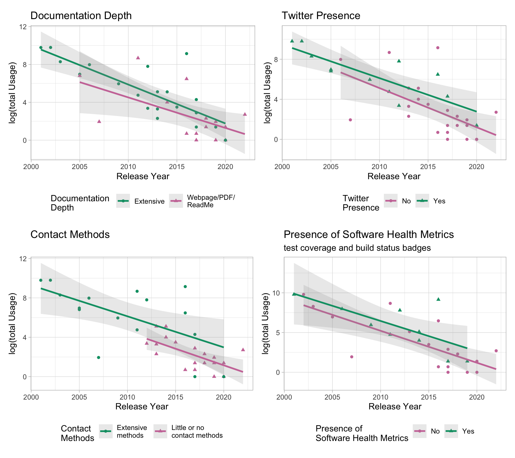

ggsave("logUsage_stratified_2x2.png", plot = p, dpi = 300, width = 8, height = 8, units = "in")

7.2 Trend using Boxplots (stratified by data type)

## Do this using box plots as discussed
# regdat %>% filter(!is.na(dataType)) %>%
#   ggplot(aes(x = releaseYear, y = log(Usage), col = extensiveContact)) +
#   geom_point(aes(shape = extensiveContact), show.legend = F) +
#   geom_smooth(method = "lm", se = T, alpha = 0.2) +
#   facet_wrap(~fct_infreq(dataType), scales = "free") +
#   labs(x = "Release Year", y = "log(total Usage)",
#        col = "Twitter Presence", shape = "Twitter \nPresence",
#        title = "Twitter Presence across data types") +
#   scale_color_manual(values = c("#CC79A7", "#009E73")) +
#   theme_light() +
#   theme(strip.background =element_rect(fill="steelblue4"),
#         strip.text = element_text(colour = 'white', size = 11),
#         panel.grid = element_blank(),
#         legend.position = "bottom")

regdat %>% 
  filter(!is.na(releaseYear) & !is.na(dataType)) %>% 
  #mutate(Year = cut(releaseYear, breaks = c(2000, 2010, 2015, 2018, 2022))) %>% 
  mutate(Year = cut(releaseYear, breaks = c(2001, 2011, 2016, 2022), include.lowest = T)) %>% 
  #mutate(Year = cut_number(releaseYear, n = 2)) %>% #count(Year)
  ggplot(aes(x = Year, y = log(Usage), fill = Year)) + 
  geom_boxplot(width = .6) +
  stat_summary(fun = "median", geom = "line", aes(group = 1), 
               lty = "dashed", lwd = .7) +
  facet_wrap(~fct_infreq(dataType)) +
  scale_color_manual(values = c("#CC79A7", "#009E73", "#E69F00", "#56B4E9")) +
  scale_fill_manual(values = c("#CC79A7", "#009E73", "#E69F00", "#56B4E9")) +
  theme_light() + 
  theme(strip.background =element_rect(fill="steelblue4"),
        strip.text = element_text(colour = 'white', size = 10),
        panel.grid = element_blank(),
        legend.position = "bottom")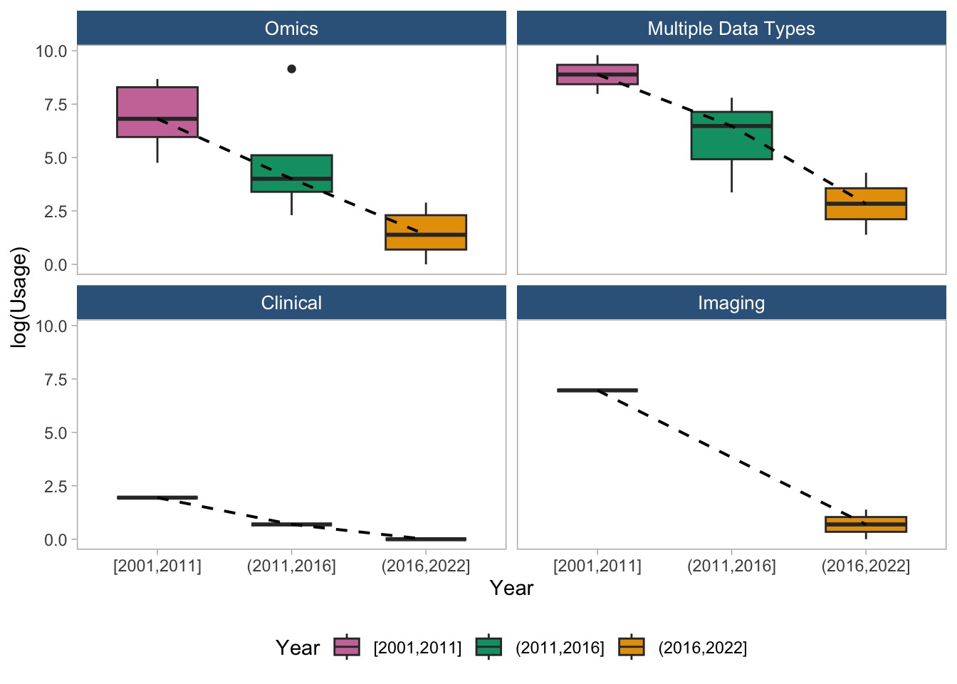

7.3 Trend using Boxplots (stratified by tool type most mature tool)

regdat %>% 
  filter(!is.na(releaseYear) & !is.na(dataType)) %>% 
  #mutate(Year = cut(releaseYear, breaks = c(2000, 2010, 2015, 2018, 2022))) %>% 
  mutate(Year = cut(releaseYear, breaks = c(2001, 2011, 2016, 2022), include.lowest = T)) %>% 
  #mutate(Year = cut_number(releaseYear, n = 2)) %>% #count(Year)
  ggplot(aes(x = Year, y = log(Usage), fill = Year)) + 
  geom_boxplot(width = .6) +
  stat_summary(fun = "median", geom = "line", aes(group = 1), 
               lty = "dashed", lwd = .7) +
  facet_wrap(~fct_infreq(toolType), nrow = 2) +
  scale_color_manual(values = c("#CC79A7", "#009E73", "#E69F00", "#56B4E9")) +
  scale_fill_manual(values = c("#CC79A7", "#009E73", "#E69F00", "#56B4E9")) +
  theme_light() + 
  theme(strip.background = element_rect(fill="steelblue4"),
        strip.text = element_text(colour = 'white', size = 10),
        panel.grid = element_blank(),
        legend.position = "bottom",
        axis.text.x = element_blank())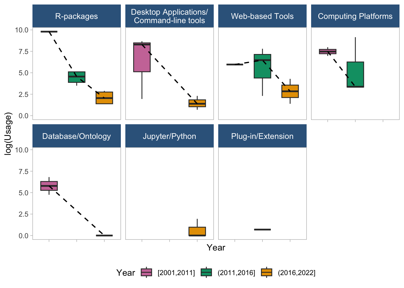

7.4 Trend using “total Usage” (facet by data types)

# Twitter

d1 <- regdat %>% filter(!is.na(dataType)) %>% 
  ggplot(aes(x = releaseYear, y = log(Usage), col = socialMedia)) + 
  geom_point(aes(shape = socialMedia)) + 
  geom_smooth(method = "lm", se = T, alpha = 0.2) +
  facet_wrap(~fct_infreq(dataType)) + 
  labs(x = "Release Year", y = "log(total Usage)", col = "Twitter \nPresence", shape = "Twitter \nPresence", 
       title = "Twitter Presence") +
  scale_color_manual(values = c("#009E73", "#CC79A7")) +
  theme_light() + 
  theme(strip.background = element_rect(fill="steelblue4"),
        strip.text = element_text(colour = 'white', size = 10),
        panel.grid = element_blank(),
        legend.position = "bottom",
        axis.text.x = element_blank())

## DocuDepth
d2 <- regdat %>% filter(!is.na(dataType)) %>% 
  ggplot(aes(x = releaseYear, y = log(Usage), col = DocuDepth)) + 
  geom_point(aes(shape = DocuDepth)) + 
  geom_smooth(method = "lm", se = T, alpha = 0.2) +
  facet_wrap(~fct_infreq(dataType)) + 
  labs(x = "Release Year", y = "log(total Usage)", col = "Documentation \nDepth", shape = "Documentation \nDepth", title = "Documentation Depth") +
  scale_color_manual(values = c("#009E73", "#CC79A7")) +
  theme_light() + 
  theme(strip.background = element_rect(fill="steelblue4"),
        strip.text = element_text(colour = 'white', size = 10),
        panel.grid = element_blank(),
        legend.position = "bottom",
        axis.text.x = element_blank())

# extensiveContact
d3 <- regdat %>% 
  mutate(extensiveContact = if_else(extensiveContact == "None", "Little or no \ncontact methods", "Extensive \nmethods")) %>% filter(!is.na(dataType)) %>% 
  ggplot(aes(x = releaseYear, y = log(Usage), col = extensiveContact)) + 
  geom_point(aes(shape = extensiveContact)) + 
  geom_smooth(method = "lm", se = T, alpha = 0.2) +
  facet_wrap(~fct_infreq(dataType)) + 
  labs(x = "Release Year", y = "log(total Usage)", col = "Contact \nMethods", shape = "Contact \nMethods", 
       title = "Contact Methods") +
  scale_color_manual(values = c("#009E73", "#CC79A7")) +
  theme_light() + 
  theme(strip.background = element_rect(fill="steelblue4"),
        strip.text = element_text(colour = 'white', size = 10),
        panel.grid = element_blank(),
        legend.position = "bottom",
        axis.text.x = element_blank())

# health metrics
d5 <- regdat %>% drop_na(simple_health_metrics) %>% filter(!is.na(dataType)) %>% 
  ggplot(aes(x = releaseYear, y = log(Usage), col = simple_health_metrics)) + 
  geom_point(aes(shape = simple_health_metrics)) + 
  geom_smooth(method = "lm", se = T, alpha = 0.2) +
  facet_wrap(~fct_infreq(dataType)) + 
  labs(x = "Release Year", y = "log(total Usage)", col = "Presence of \nSoftware Health Metrics", shape = "Presence of \nSoftware Health Metrics", 
       title = "Presence of Software Health Metrics", subtitle = ("test coverage and build status badges")) + scale_color_manual(values = c("#CC79A7", "#009E73")) +
  theme_light() + 
  theme(strip.background = element_rect(fill="steelblue4"),
        strip.text = element_text(colour = 'white', size = 10),
        panel.grid = element_blank(),
        legend.position = "bottom",
        axis.text.x = element_blank())

p2 <- (d2 + d1) / (d3 + d5)
p2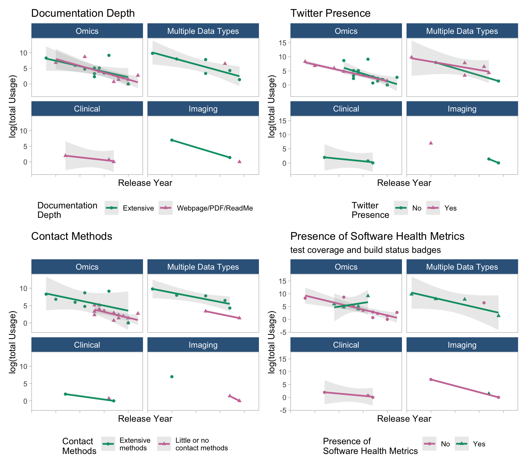

8. Trend using “total Mentions”

# Twitter
d1 <- regdat %>% 
  ggplot(aes(x = releaseYear, y = log(totalMentions), col = socialMedia)) + 
  geom_point(aes(shape = socialMedia)) + 
  geom_smooth(method = "lm", se = T, alpha = 0.2) +
  labs(x = "Release Year", y = "log(total Mentions)", col = "Twitter \nPresence", shape = "Twitter \nPresence", title = "Twitter Presence") +
  scale_color_manual(values = c("#009E73", "#CC79A7")) +
  theme_light() + 
  coord_equal() + 
  theme(legend.position = "bottom",
        aspect.ratio = .6)

## DocuDepth
d2 <- regdat %>%
  mutate(DocuDepth = fct_recode(DocuDepth, "Webpage/PDF/\nReadMe" = "Webpage/PDF/ReadMe")) %>% 
  ggplot(aes(x = releaseYear, y = log(totalMentions), col = DocuDepth)) + 
  geom_point(aes(shape = DocuDepth)) + 
  geom_smooth(method = "lm", se = T, alpha = 0.2) +
  labs(x = "Release Year", y = "log(total Mentions)", col = "Documentation \nDepth", shape = "Documentation \nDepth", title = "Documentation Depth") +
  scale_color_manual(values = c("#009E73", "#CC79A7")) +
  theme_light() + 
  coord_equal() + 
  theme(legend.position = "bottom",
        aspect.ratio = .6)

# extensiveContact
d3 <- regdat %>% mutate(extensiveContact = if_else(extensiveContact == "None", "Little or no \ncontact methods", "Extensive \nmethods")) %>% 
  ggplot(aes(x = releaseYear, y = log(totalMentions), col = extensiveContact)) + 
  geom_point(aes(shape = extensiveContact)) + 
  geom_smooth(method = "lm", se = T, alpha = 0.2) +
  labs(x = "Release Year", y = "log(total Mentions)", col = "Contact \nMethods", shape = "Contact \nMethods", title = "Contact Methods") +
  scale_color_manual(values = c("#009E73", "#CC79A7")) +
  theme_light() + 
  coord_equal() + 
  theme(legend.position = "bottom",
        aspect.ratio = .6)

# CiteHow
d4 <- regdat %>% 
  ggplot(aes(x = releaseYear, y = log(totalMentions), col = citeHow)) + 
  geom_point(aes(shape = citeHow)) + 
  geom_smooth(method = "lm", se = T, alpha = 0.2) +
  labs(x = "Release Year", y = "log(total Mentions)", subtitle = "Information for citing software") +
  scale_color_manual(values = c("#009E73", "#CC79A7")) +
  theme_light() + 
  coord_equal() + 
  theme(legend.position = "bottom",
        aspect.ratio = .6)

# health metrics
d5 <- regdat %>% drop_na(simple_health_metrics) %>%
  ggplot(aes(x = releaseYear, y = log(totalMentions), col = simple_health_metrics)) + 
  geom_point(aes(shape = simple_health_metrics)) + 
  geom_smooth(method = "lm", se = T, alpha = 0.2) +
  labs(x = "Release Year", y = "log(total Mentions)", col = "Presence of \nSoftware Health Metrics", shape = "Presence of \nSoftware Health Metrics", 
       title = "Presence of Software Health Metrics", subtitle = ("test coverage and build status badges")) + scale_color_manual(values = c("#CC79A7", "#009E73")) +
  theme_light() + 
  coord_equal() + 
  theme(legend.position = "bottom",
        aspect.ratio = .6)

p2 <- (d2 + d1) / (d3 + d5)
p2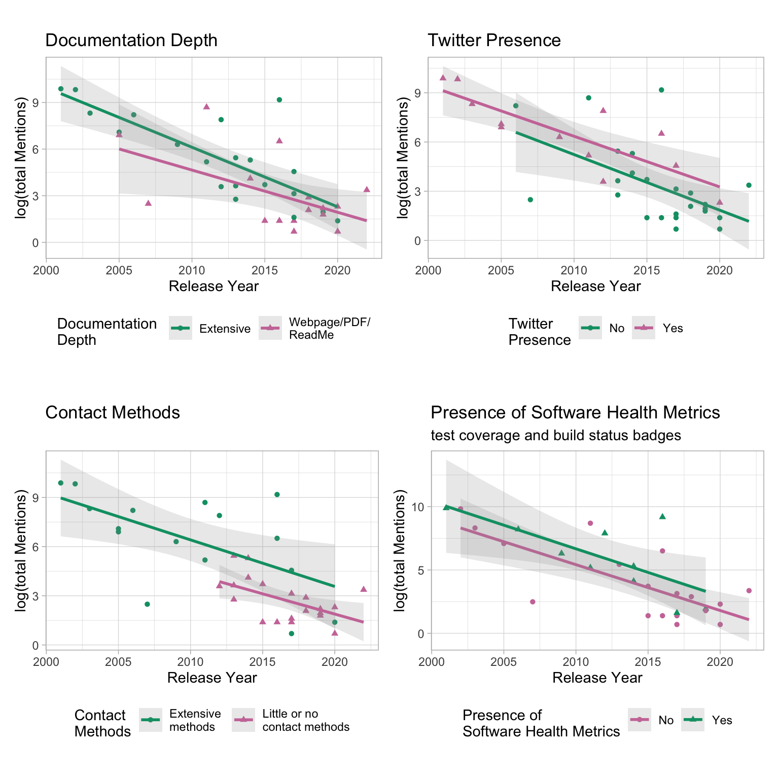

ggsave("logMentions_stratified_2x2.png", plot = p2, dpi = 300, width = 8, height = 8, units = "in")

The trends are similar whether using total Mentions or just Usage as the response variable.

Infrastructure and Citation Analysis

Awan Afiaz - Graduate Student

2023-05-29